16. Knapsack Problems, Dynamic Programming, and Graph Optimization Problems#
Today#
- Part I: Knapsack Problems
- Part II: Graph Optimization Problems
Knapsack Problems#
Given a set of items, each with a weight and a value, determine the number of each item to include in a collection so that the total weight is less than or equal to a given limit and the total value is as large as possible.
Example#
A burglar who has a knapsack that can hold at most 20 kg of loot breaks into a house and finds the items as shown below. Obviously, he will not be able to take all of the items, so he needs to decide what to take and what to leave behind.
Item
Value
Weight
Value/Weight
Book
10
1
10
Violin
175
10
17.5
Camera
50
2
25
TV
200
20
10
Painting
90
9
10
Wine
20
4
5
The question becomes, what combination will bring him the greatest wealth?
Greedy Algorithms#
The simplest way to find an approximate solution to this problem. Choose the best item first, then the next best, and continue until reached the limit.
What is the best meaning? Is it the most valuable, least weight, or the best value/weight ratio?
For example, the following results show three different solutions via greedy algorithms.
Greedy-by-value:
No.
Item to be take
Cummulative value
Cummulative weight
1
TV
200
20
Greedy-by-weight-inverse:
No.
Item to be take
Cummulative value
Cummulative weight
1
Book
10
1
2
Camera
60
3
3
Wine
80
7
4
Painting
170
16
Greedy-by-ratio
No.
Item to be take
Cummulative value
Cummulative weight
1
Camera
50
2
2
Violin
225
12
3
Book
235
13
4
Wine
255
17
Greedy algorithm can provide an approximate solution with efficiency, but NOT guarantee to find the optimal solution.
Implementation of Greedy Algorithms#
from scripts.part1.testFuncs import test1

test1()
Use greedy by value to fill knapsack of size 20
Total value of items taken is 200.0.
    <TV, 200, 20>
Use greedy by weight to fill knapsack of size 20
Total value of items taken is 170.0.
    <book, 10, 1>
    <camera, 50, 2>
    <wine, 20, 4>
    <painting, 90, 9>
Use greedy by density to fill knapsack of size 20
Total value of items taken is 255.0.
    <camera, 50, 2>
    <violin, 175, 10>
    <book, 10, 1>
    <wine, 20, 4>
test1(25)
Use greedy by value to fill knapsack of size 25
Total value of items taken is 260.0.
    <TV, 200, 20>
    <camera, 50, 2>
    <book, 10, 1>
Use greedy by weight to fill knapsack of size 25
Total value of items taken is 170.0.
    <book, 10, 1>
    <camera, 50, 2>
    <wine, 20, 4>
    <painting, 90, 9>
Use greedy by density to fill knapsack of size 25
Total value of items taken is 325.0.
    <camera, 50, 2>
    <violin, 175, 10>
    <book, 10, 1>
    <painting, 90, 9>
Exercise#
Item |
Value |
Weight |
Value/Weight |
Easy to Sale |
|---|---|---|---|---|
Book |
10 |
1 |
10 |
1 |
Violin |
175 |
10 |
17.5 |
7 |
Camera |
50 |
2 |
25 |
2 |
TV |
200 |
20 |
10 |
10 |
Painting |
90 |
9 |
10 |
9 |
Wine |
20 |
4 |
5 |
1 |
Use greedy algorithm to find the solution
The 0/1 Knapsack Problems#
Each item is represented by a pair, \(<value, weight>\)
The knapsack can accommodate items with a total weight of no more than \(w\).
A vector \(I\) of length \(n\) represents the set of available items. Each element of the vector is an item.
A vector \(V\) of length \(n\) represents whether each item is taken or not (e.g. \(V[i] = 1\) represents that item \(I[i]\) is taken).
Find the optimal \(V\) that
Brute-force Search Method (Exhaustive Enumeration)#
Enumerate all possible combinations of items.
Remove all of the combinations which does not meet the constraints.
Choose the combination whose value is the largest from the remaining.
Implementation#
from scripts.part1.testFuncs import test2, test3

test2()
Total value of items taken is 275.0
<book, 10, 1>
<violin, 175, 10>
<painting, 90, 9>
test2(15)
Total value of items taken is 235.0
<book, 10, 1>
<violin, 175, 10>
<camera, 50, 2>
test3(numItems=20)
Total value of items taken is 799.0
<0, 27, 1>
<2, 82, 4>
<8, 144, 5>
<12, 48, 2>
<13, 166, 4>
<14, 169, 2>
<15, 163, 1>
Brief Summary#
It’s simple but time-consuming. The computational complexity is \(O(n \cdot 2^n)\).
It can definitely find the optimal solution.
Dynamic Programming#
“The fact that I was really doing mathematics… was something not even a Congressman could object to.”
... Richard Bellman on the Birth of Dynamic Programming
What is Dynamic Programming?#
A method for efficiently solving problems that exhibit the characteristics of overlapping subproblems and optimal structure.
A problems has optimal structure if a globally optimal solution can be found by combining optimal solutions to local subproblems. Ex: Merge sort
A problem has overlapping subproblems if an optimal solution involves solving the same problem multiple times.
The key idea behind dynamic programming is memorization.
A Simple Example: Fibonacci#
def fib(n):
    if n==0 or n==1:
        return 1
    else:
        return fib(n-1) + fib(n-2)

def fastFib(n, memo={}):
    if n==0 or n==1:
        return 1
    try:
        return memo[n]
    except KeyError:
        result = fastFib(n-1, memo) + fastFib(n-2, memo)
        memo[n] = result
        return result
Dynamic Programming and the 0/1 Knapsack Problems#
Dynamic programming provides a practical method for solving the 0/1 knapsack problems in a reasonable amount of time.
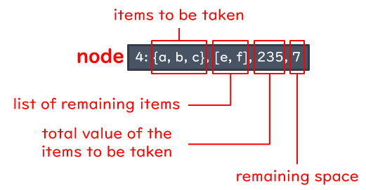
The key idea is to think about exploring the space of possible solutions by constructing a rooted binary tree that enumerates all states that satisfy the constraint.
Rooted Binary Tree#
Item |
Value |
Weight |
Value/Weight |
|
|---|---|---|---|---|
a |
Book |
10 |
1 |
10 |
b |
Violin |
175 |
10 |
17.5 |
c |
Camera |
50 |
2 |
25 |
d |
TV |
200 |
20 |
10 |
e |
Painting |
90 |
9 |
10 |
f |
Wine |
20 |
4 |
5 |
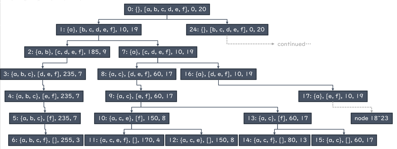
There is exactly one node without any parent. This node is called the root.
Each non-root node has exactly one parent.
Each node has at most two children. A childless node is called a leaf.
Implementation#
from scripts.part1.testFuncs import testDT1

testDT1()
testDT1(10)
testDT1(20)
Decision Tree Test 1 (max. weight = 5):
    Items taken:
         <camera, 50, 2>
         <book, 10, 1>
    Total value of items taken = 60
Decision Tree Test 1 (max. weight = 10):
    Items taken:
         <violin, 175, 10>
    Total value of items taken = 175
Decision Tree Test 1 (max. weight = 20):
    Items taken:
         <painting, 90, 9>
         <violin, 175, 10>
         <book, 10, 1>
    Total value of items taken = 275
from scripts.part1.testFuncs import testDT2

testDT2()
testDT2(20, 16)
testDT2(20, 128)
Decision Tree Test 2 (max. weight = 5):
    Items taken:
         <1, 151, 3>
    Total value of items taken = 151
Decision Tree Test 2 (max. weight = 20):
    Items taken:
         <12, 76, 4>
         <9, 167, 4>
         <7, 166, 8>
    Total value of items taken = 409
Decision Tree Test 2 (max. weight = 20):
    Items taken:
         <102, 36, 1>
         <50, 134, 3>
         <43, 133, 1>
         <42, 76, 2>
         <39, 124, 2>
         <34, 117, 2>
         <29, 132, 2>
         <26, 178, 4>
         <11, 170, 3>
    Total value of items taken = 1100
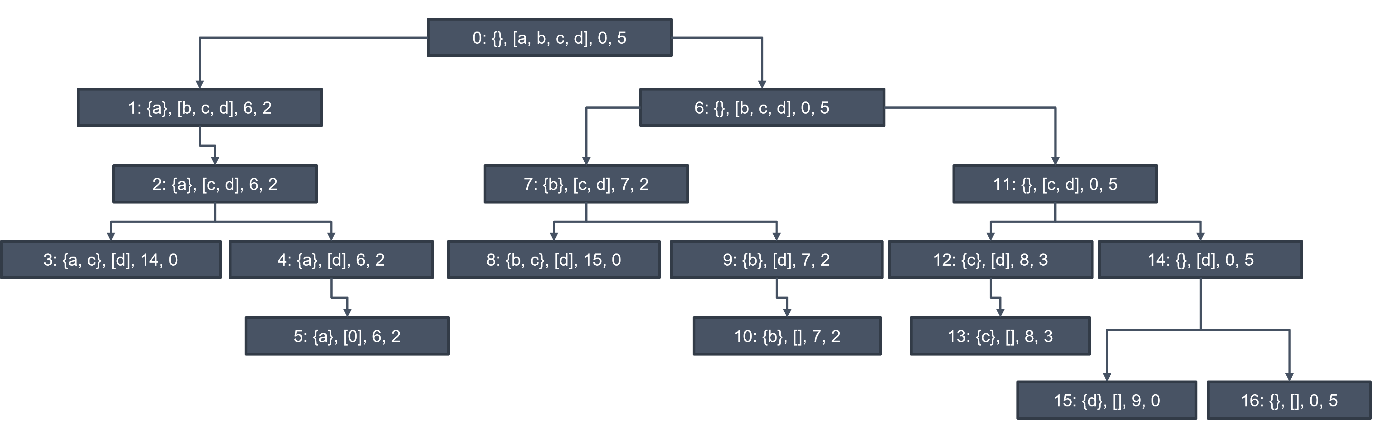
Considering another situation
Item |
Value |
Weight |
|---|---|---|
a |
6 |
3 |
b |
7 |
3 |
c |
8 |
2 |
d |
9 |
5 |
The decision tree becomes
Dynamic Programming Solution#
from scripts.part1.testFuncs import testDT3

testDT3(20, 128)
Decision Tree Test 2 (max. weight = 20):
    Items taken:
         <101, 152, 2>
         <91, 174, 4>
         <89, 186, 4>
         <83, 181, 1>
         <71, 187, 3>
         <53, 149, 1>
         <39, 97, 1>
         <31, 119, 3>
         <6, 127, 1>
    Total value of items taken = 1372
Graph Theory#
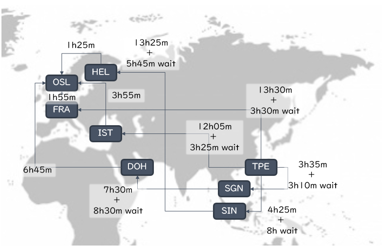
Introduction: From TPE to OSL#
What is the cheapest, fastest, or the best flight from TPE to OSL, on Mar. 30 in 2023?
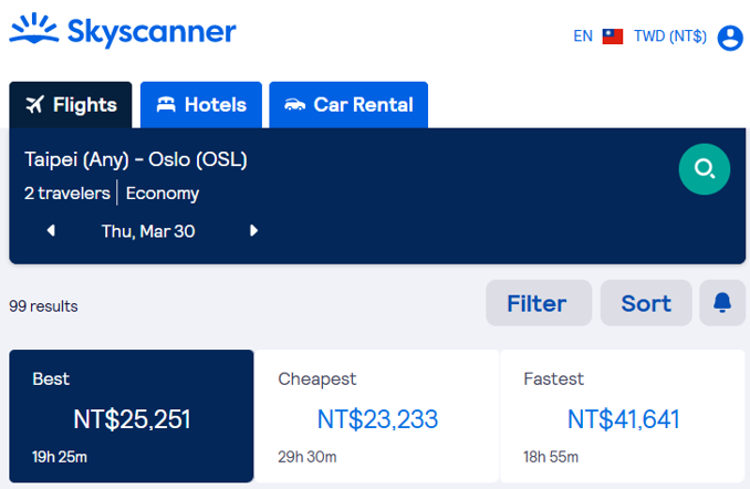
* The best choice (cost: NT$25,251):

    |Flight No.|From|To|Flight Time|Connecting Time|
    |:--:|:--:|:--:|:--:|:--:|
    |TK25|TPE|IST|12h05m|x|
    |TK1751|IST|OSL|3h55m|3h25m|

* The cheapest choice (cost: NT$23,233):

    |Flight No.|From|To|Flight Time|Connecting Time|
    |:--:|:--:|:--:|:--:|:--:|
    |CI783|TPE|SGN|3h35m|x|
    |QR971|SGN|DOH|7h30m|3h10m|
    |QR175|DOH|OSL|6h45m|8h30m|

* The fastest choice (cost: NT$41,641):

    |Flight No.|From|To|Flight Time|Connecting Time|
    |:--:|:--:|:--:|:--:|:--:|
    |CI61|TPE|FRA|13h30m|x|
    |LH860|FRA|OSL|1h55m|3h30m|
How do we calculate this?
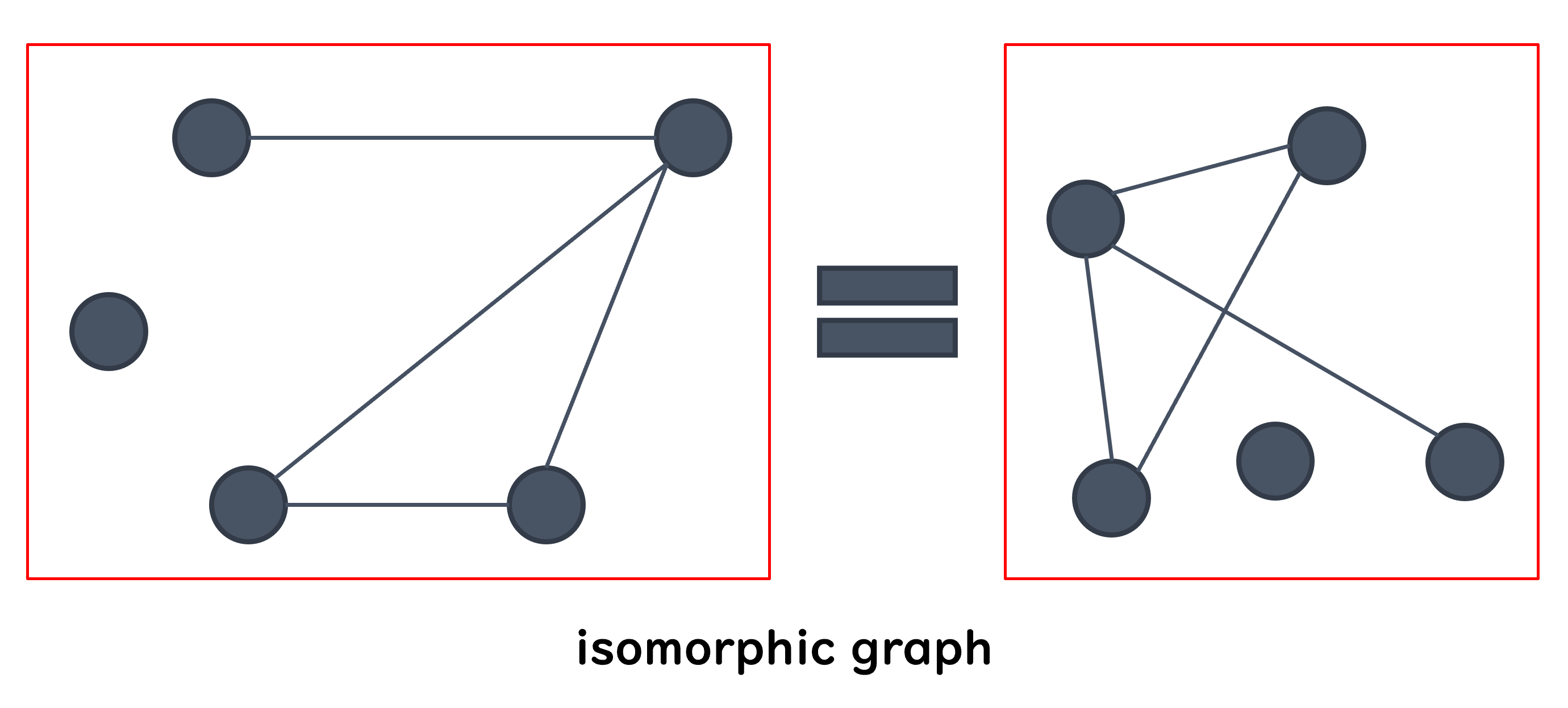
A graph is a set of objects called nodes (or vertices) connected by a set of edges (or arcs).
It is a thing that can be used to record associations and relationships.
Directed Graph (Digraph)#
If the edges are unidirectional the graph is called a directed graph or digraph.
In a directed graph, if there is an edge from node \(n_1\) to node \(n_2\), we refer to \(n_1\) as the source or parent node and \(n_2\) as the destination or child node.

Weighted Graph#
If a weight is associated with each edge in a graph or digraph, it is called a weighted graph.
Common Data Structures of Graph#
Edge List#
Simple, intuitive, and low spatial complexity
Difficult for computation - not easy to find all edges that connected with a single node.
#
0
1
2
3
4
5
6
7
8
9
Source
TPE
TPE
TPE
TPE
SGN
SIN
IST
FRA
DOH
HEL
Destination
SGN
SIN
IST
FRA
DOH
HEL
OSL
OSL
OSL
OSL
Adjacency Matrix#
Clear but high spatial complexity, \(O(n \times n)\)
Adjacency matrix of a digraph
#
TPE
SGN
SIN
IST
DOH
FRA
HEL
OSL
TPE
0
1
1
1
0
1
0
0
SGN
0
0
0
0
1
0
0
0
SIN
0
0
0
0
0
0
1
0
IST
0
0
0
0
0
0
0
1
DOH
0
0
0
0
0
0
0
1
FRA
0
0
0
0
0
0
0
1
HEL
0
0
0
0
0
0
0
1
OSL
0
0
0
0
0
0
0
0
Adjacency matrix of a weighted digraph (\(\text{weight} = \text{flight time} + \text{connecting time}\))
#
TPE
SGN
SIN
IST
DOH
FRA
HEL
OSL
TPE
0
405
745
930
0
1020
0
0
SGN
0
0
0
0
960
0
0
0
SIN
0
0
0
0
0
0
1150
0
IST
0
0
0
0
0
0
0
235
DOH
0
0
0
0
0
0
0
405
FRA
0
0
0
0
0
0
0
115
HEL
0
0
0
0
0
0
0
85
OSL
0
0
0
0
0
0
0
0
Adjacency matrix of a graph
#
TPE
SGN
SIN
IST
DOH
FRA
HEL
OSL
TPE
0
1
1
1
0
1
0
0
SGN
1
0
0
0
1
0
0
0
SIN
1
0
0
0
0
0
1
0
IST
1
0
0
0
0
0
0
1
DOH
0
1
0
0
0
0
0
1
FRA
1
0
0
0
0
0
0
1
HEL
0
0
1
0
0
0
0
1
OSL
0
0
0
1
1
1
1
0
Adjacency List#
Less spatial complexity in some cases.
Node
Edges
Weights
TPE
[SGN, SIN, IST, FRA][405, 745, 930, 1020]SGN
[DOH,][960,]SIN
[HEL,][1150,]IST
[OSL,][235,]DOH
[OSL,][405,]FRA
[OSL,][115,]HEL
[OSL,][85,]OSL
[][]
Graph Optimization Problems#
Shortest path
Shortest weighted path
Maximum clique
Min cut
…
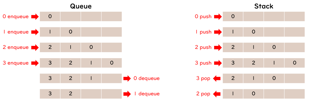
Queue and Stack#
Queue: First In First Out (FIFO)
Stack: Last In First Out (LIFO)
Breadth-First Search (BFS)#
A graph travesal algorithm that prioritizes the expansion of breadth
Start from the initial node
Enqueue the initial node
Repeat the following steps until nothing remaining in the queue:
Dequeue the first item from queue
Enqueue the unvisited neighbors (in the order of index) of the node
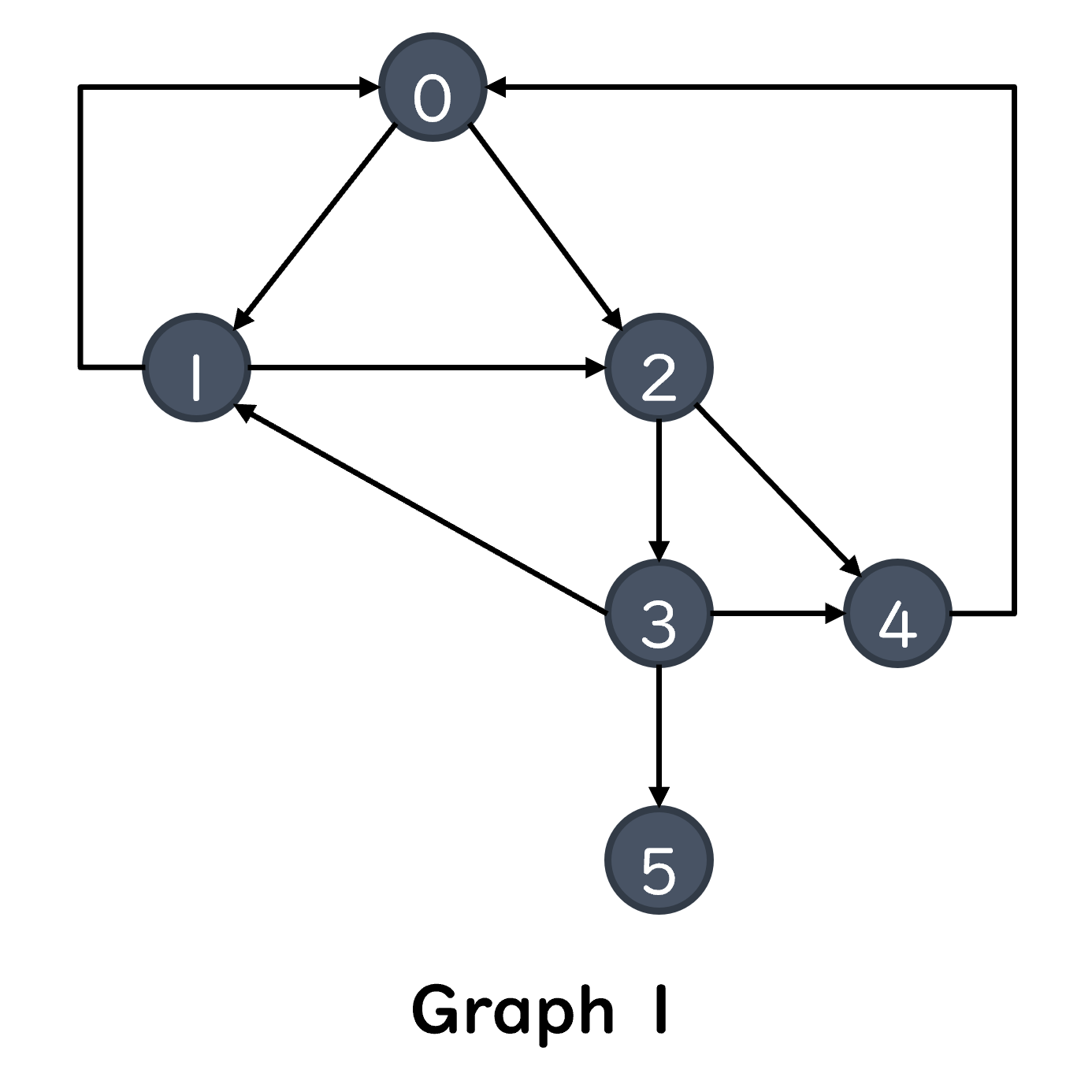
Example 1: Find All Paths from Node 0 to Node 1#
# of Iteration |
Status of Queue |
Dequeue the First Item |
Enqueue the Result |
End of This Round |
|---|---|---|---|---|
0 |
|
|
|
|
1 |
|
|
|
|
2 |
|
|
|
|
3 |
|
|
|
|
4 |
|
|
|
|
5 |
|
|
X |
|
6 |
|
|
|
|
7 |
|
|
X |
|
8 |
|
|
X |
|
9 |
|
|
X |
|
10 |
|
|
X |
|
11 |
|
|
X |
|
12 |
|
|
X |
X |
from scripts.part2.testFuncs import test1

test1()
Current BFS path: 0
Current BFS path: 0->1
Current BFS path: 0->2
Current BFS path: 0->1->2
Current BFS path: 0->2->3
Current BFS path: 0->2->4
Current BFS path: 0->1->2->3
Current BFS path: 0->1->2->4
Current BFS path: 0->2->3->4
Current BFS path: 0->2->3->5
Current BFS path: 0->2->3->1
Current BFS path: 0->1->2->3->4
Current BFS path: 0->1->2->3->5
Result of BFS:
 ['0->2->3->5', '0->1->2->3->5']
Shortest path:
 0->2->3->5, path length = 3
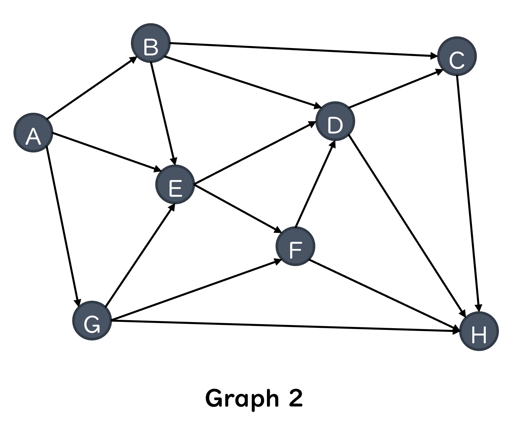
Example 2: Find All Paths from A to H#
# of Iteration |
Status of Queue |
Dequeue the First Item |
Enqueue the Result |
End of This Round |
|---|---|---|---|---|
0 |
|
|
|
|
1 |
|
|
|
|
2 |
|
|
|
|
3 |
|
|
|
|
4 |
|
|
|
\(\vdots\) |
\(\vdots\) |
\(\vdots\) |
\(\vdots\) |
\(\vdots\) |
from scripts.part2.testFuncs import test2

test2()
Current BFS path: A
Current BFS path: A->B
Current BFS path: A->E
Current BFS path: A->G
Current BFS path: A->B->C
Current BFS path: A->B->D
Current BFS path: A->B->E
Current BFS path: A->E->D
Current BFS path: A->E->F
Current BFS path: A->G->E
Current BFS path: A->G->F
Current BFS path: A->G->H
Current BFS path: A->B->C->H
Current BFS path: A->B->D->C
Current BFS path: A->B->D->H
Current BFS path: A->B->E->D
Current BFS path: A->B->E->F
Current BFS path: A->E->D->C
Current BFS path: A->E->D->H
Current BFS path: A->E->F->D
Current BFS path: A->E->F->H
Current BFS path: A->G->E->D
Current BFS path: A->G->E->F
Current BFS path: A->G->F->D
Current BFS path: A->G->F->H
Current BFS path: A->B->D->C->H
Current BFS path: A->B->E->D->C
Current BFS path: A->B->E->D->H
Current BFS path: A->B->E->F->D
Current BFS path: A->B->E->F->H
Current BFS path: A->E->D->C->H
Current BFS path: A->E->F->D->C
Current BFS path: A->E->F->D->H
Current BFS path: A->G->E->D->C
Current BFS path: A->G->E->D->H
Current BFS path: A->G->E->F->D
Current BFS path: A->G->E->F->H
Current BFS path: A->G->F->D->C
Current BFS path: A->G->F->D->H
Current BFS path: A->B->E->D->C->H
Current BFS path: A->B->E->F->D->C
Current BFS path: A->B->E->F->D->H
Current BFS path: A->E->F->D->C->H
Current BFS path: A->G->E->D->C->H
Current BFS path: A->G->E->F->D->C
Current BFS path: A->G->E->F->D->H
Current BFS path: A->G->F->D->C->H
Current BFS path: A->B->E->F->D->C->H
Current BFS path: A->G->E->F->D->C->H
Result of BFS:
 ['A->G->H', 'A->B->C->H', 'A->B->D->H', 'A->E->D->H', 'A->E->F->H', 'A->G->F->H', 'A->B->D->C->H', 'A->B->E->D->H', 'A->B->E->F->H', 'A->E->D->C->H', 'A->E->F->D->H', 'A->G->E->D->H', 'A->G->E->F->H', 'A->G->F->D->H', 'A->B->E->D->C->H', 'A->B->E->F->D->H', 'A->E->F->D->C->H', 'A->G->E->D->C->H', 'A->G->E->F->D->H', 'A->G->F->D->C->H', 'A->B->E->F->D->C->H', 'A->G->E->F->D->C->H']
Shortest path:
 A->G->H, path length = 2
Depth-First Search (DFS)#
A graph travesal algorithm that prioritizes the expansion of depth
Start from the initial node
Go to the farthest node from the starting node first
Using the concept of stack
Can be achieved recursively
Example 3: Find All Paths from A to H (DFS)#
# of Recursive Calls |
Status of Stack |
Found Node |
Leaf? |
Result |
|---|---|---|---|---|
0 |
|
|
|
|
1 |
|
|
|
|
2 |
|
|
|
|
3 |
|
|
|
|
4 |
|
|
|
|
5 |
|
|
|
|
6 |
|
|
|
|
7 |
|
|
|
|
\(\vdots\) |
\(\vdots\) |
\(\vdots\) |
\(\vdots\) |
\(\vdots\) |
Run the script:
python main_Lecture01.py --num 3
The Shortest Path of Weighted Graph#
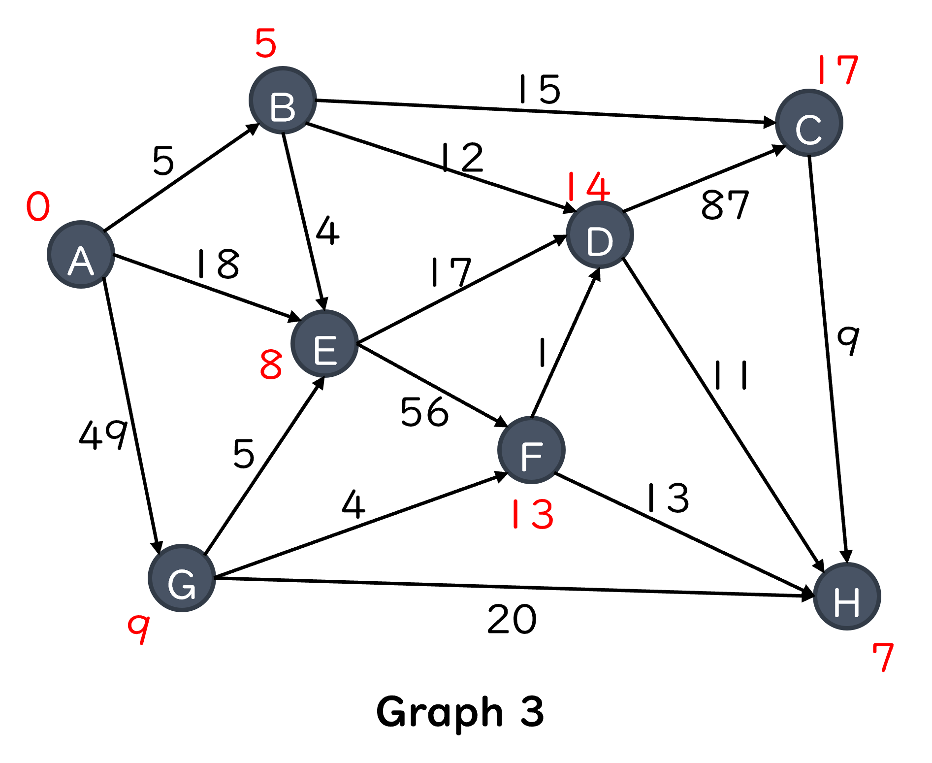
Example 4: Find the Shortest Path from A to H (BFS or DFS)#
Run this on terminal:
BFS:
python main_Lecture01.py --num 5
DFS:
python main_Lecture01.py --num 6
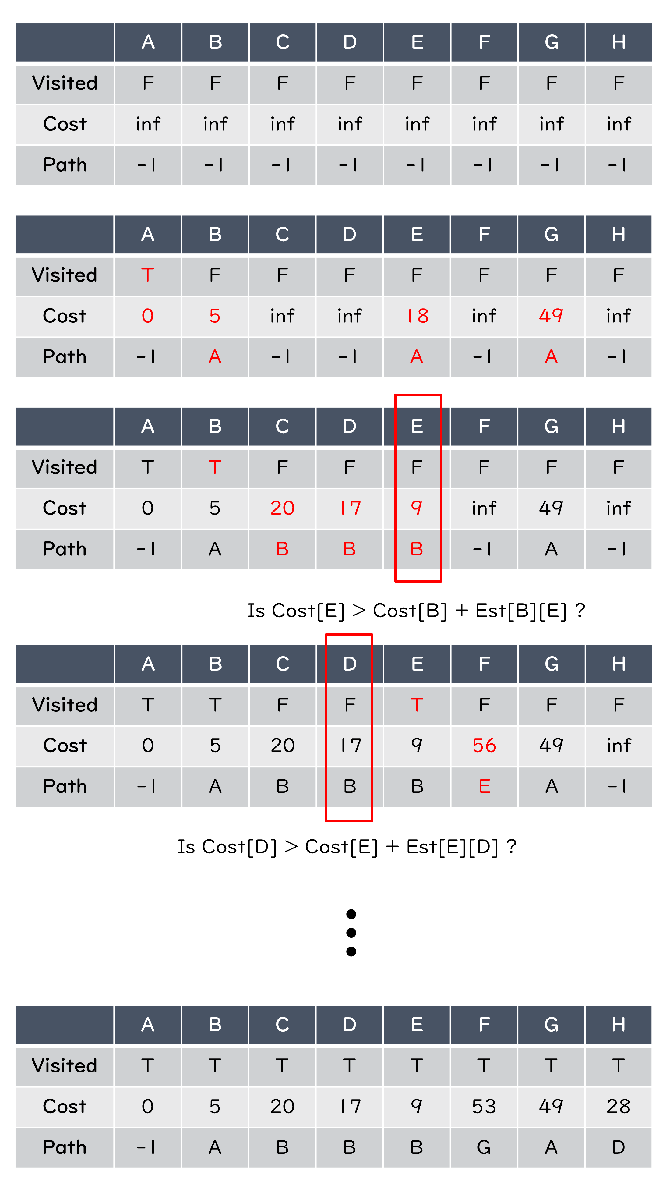
Dijkstra Algorithm#
An algorithm that calculates the shortest paths from a specific node to all other nodes of a graph
Create a table to record three things at the beginning,
Visited: has this node been visited? (default:
False)Cost: path length from source node to current node (default:
infinite)Path: previous connected node of this node (default:
-1)
Algorithm:
Start from the source node
Update the cost and path
Choose the nearest unvisited node as the next
Example: Find the shortest paths from node A to the others#