11. Simple Numerical Algorithms II

Last time

• How to evaluate the efficiency of your algorithm?

• Orders of growth and big Oh notation

• Searching algorithms

Today

• Searching algorithms
• Sorting algorithms
• Lambda
• Hash table

Searching algorithms

1. Searching an element in an UNSORTED list

   def searchEx(L, target):
       exist = False
       for i in range(len(L)):
           if L[i] == target:
               exist = True
               break
       return exist
   

   • The computational complexity of searchEx is \(O(n)\).

---

2. Searching an element in an SORTED list

   def searchEx2(L, target):
       exist = False
       for i in range(len(L)):
           if L[i] == target:
               exist = True
               break
           elif L[i] > target:
               break
       return exist
   

   • The computational complexity of searchEx2 is still \(O(n)\).

---

3. Searching an element in an SORTED list with different method

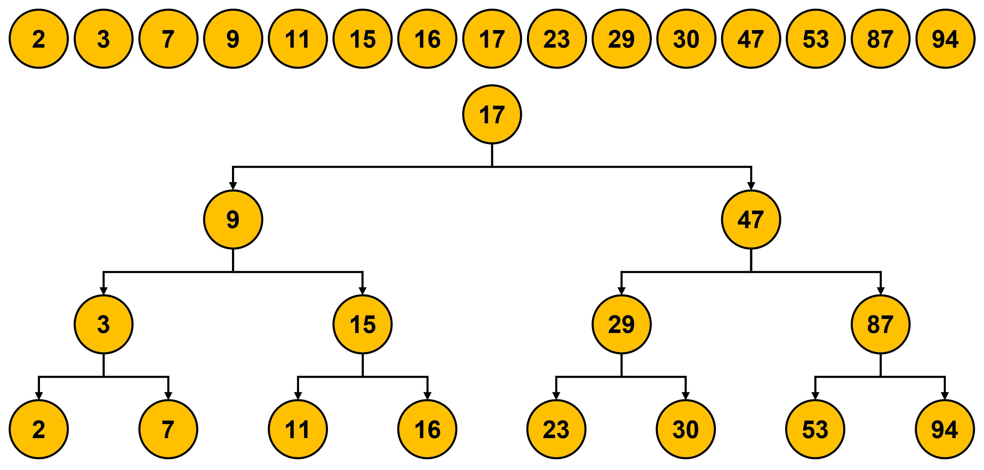
   def searchBi(L, target):
       def search(L, target, low, high):
           if high == low:
               return (L[low]==target)
           
           mid = (low + high)//2
   
           if L[mid] == target:
               return True
           
           elif L[mid] > target:
               if low == mid:
                   return False
               else:
                   return search(L, target, low, mid-1)
           
           else:
               return search(L, target, mid+1, high)
       
       if len(L) == 0:
           return False
       else:
           return search(L, target, 0, len(L)-1)
   

   • The computational complexity of searchBi is \(O(\log{n})\).

---

Should we sort the list first?

Method	Sorted?	Computational complexity
Linear search	\(\chi\)	\(O(n)\)
Linear search	\(\checkmark\)	\(O(n)\)
Bisection search	\(\checkmark\)	\(O(\log{n})\)

• Should we sort the list before we searching something?

• Assuming the computational complexity of sorting algorithm is \(O(sorting)\), the question becomes

  • Is \(O(sorting) + O(\log{n}) < O(n)\) true?

  • \(O(sorting) < O(n) - O(\log{n}) \approx O(n)\)

• The complexity of sorting algorithm is \(O(n)\) at least. It seems to be worthless if we sort the list before searching. However, sometimes we will do a lot of searches instead of searching once. In this case, the overall complexity will be different.

  • \(O(sorting) + k \cdot O(\log{n}) < k \cdot O(n)\)

Sorting algorithms

A. Monkey sort (Bogo sort)

• While list is not sorted, random shuffles the list until it is sorted.

  Cases	\(O()\)	Note
  Best case	\(O(n)\)	\(O(n)\) for checking whether it is sorted
  Average case	\(O(n \times n!)\)	\(O(n!)\) for random shuffle, \(O(n)\) for checking every time
  Worst case	\(O(\infty)\)	You never get sorted result

---

B. Bubble sort

1. Compare consecutive pairs of elements

2. Swap them such that smaller is first

3. Repeat it until no more swaps have been made in one loop

   Cases	\(O()\)	Note
   Best case	\(O(n)\)	for checking whether it is sorted
   Average case	\(O(n^2)\)	for comparison and swapping
   Worst case	\(O(n^2)\)	for comparison and swapping

   

---

C. Selection sort

1. Find the minimum element in a list

2. Swap it with the first element of list

3. Repeat it in the remaining sub-list

   Cases	\(O()\)	Note
   Best case	\(O(n^2)\)	for comparison
   Average case	\(O(n^2)\)	for comparison and swapping
   Worst case	\(O(n^2)\)	for comparison and swapping

   

---

D. Insertion sort

1. Start from the first element

2. When a new element comes in, compare and insert

3. Repeat the above steps for the remaining elements

   Cases	\(O()\)	Note
   Best case	\(O(n)\)	for comparison
   Average case	\(O(n^2)\)	for comparison and swapping
   Worst case	\(O(n^2)\)	for comparison and swapping

   

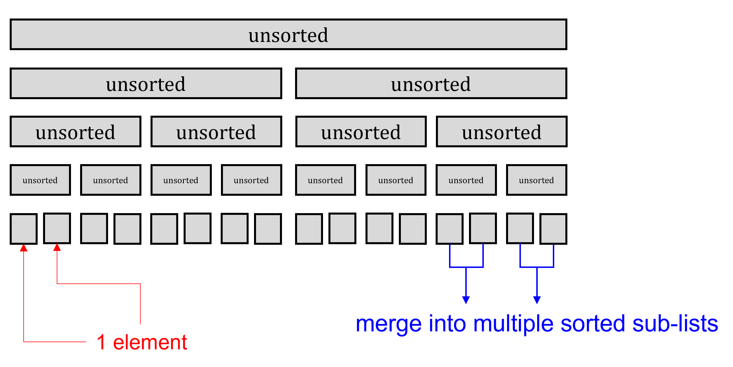
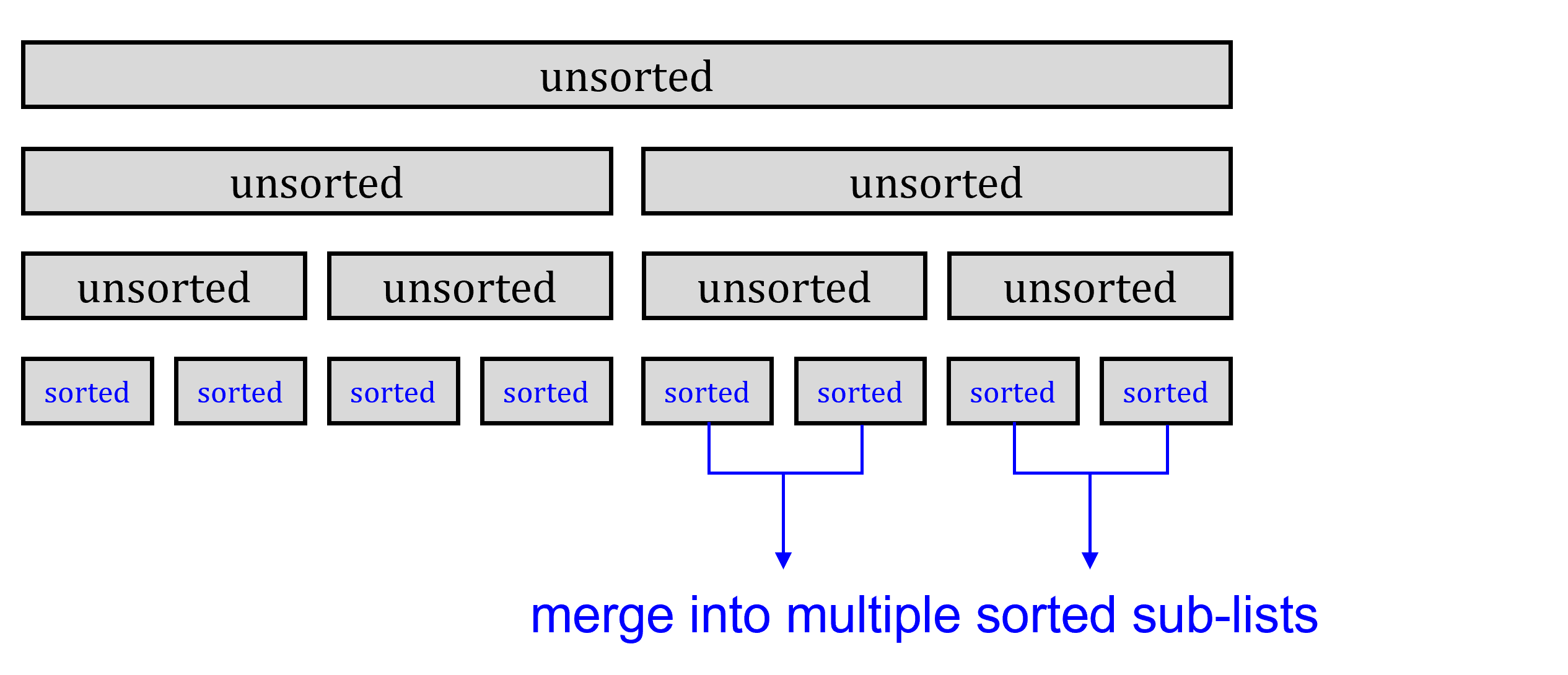
E. Merge sort

1. Recursively divide the current lists into sub-lists

2. Sort the elements of 2 sub-lists and merge into one list

3. Repeat the above steps

   Cases	\(O()\)	Note
   Best case	\(O(n\log{n})\)	for merging and sorting
   Average case	\(O(n\log{n})\)	for merging and sorting
   Worst case	\(O(n\log{n})\)	for merging and sorting

   

---

---

---

---

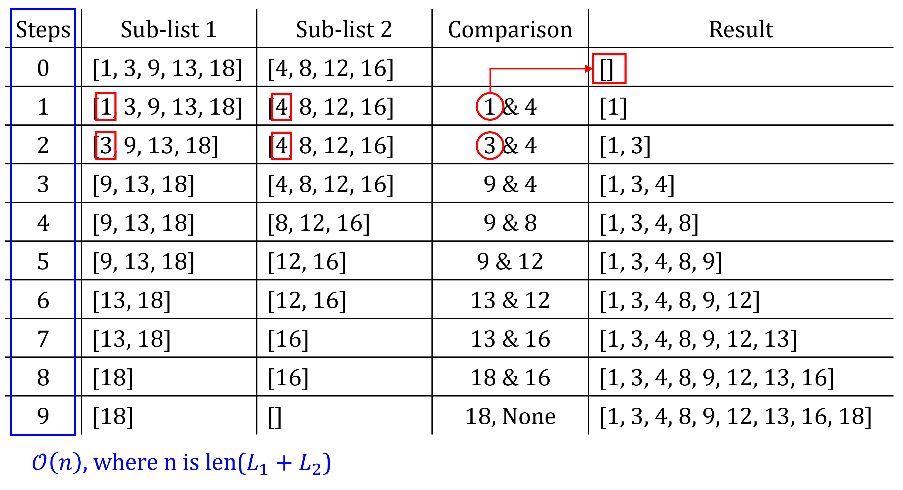
# Sample code of merge sort

def merge(L1, L2, compare):
    """
    Assumes L1 and L2 are sorted lists and compare defines an ordering on the elements.
    Returns a new sorted (by compare) list containing the same elements as (L1 + L2) would contain.
    """
    result = []
    i, j = 0, 0
    while i < len(L1) and j < len(L2):
        if compare(L1[i], L2[j]):
            result.append(L1[i])
            i += 1
        else:
            result.append(L2[j])
            j += 1
    while (i < len(L1)):
        result.append(L1[i])
        i += 1
    while (j < len(L2)):
        result.append(L2[j])
        j += 1
    return result

def mergeSort(L, compare = lambda x, y: x < y):
    """
    Assumes L is a list, compare defines an ordering on elements of L
    Returns a new sorted list with the same elements as L
    """
    if len(L) < 2:
        return L[:]
    else:
        middle = len(L)//2
        left = mergeSort(L[:middle], compare)
        right = mergeSort(L[middle:], compare)
        return merge(left, right, compare)

import random

L = []
for i in range(20):
    L.append(random.randint(-100,100))

print("L:")
print(L)
print("=="*50)
print("L ascend:")
print(mergeSort(L))
print("=="*50)
print("L descend:")
print(mergeSort(L, lambda x, y: x > y))

L:
[1, 75, 37, 40, -90, 58, 6, 21, -35, -45, -67, -98, -99, -39, -58, 6, -33, 87, -70, 14]
====================================================================================================
L ascend:
[-99, -98, -90, -70, -67, -58, -45, -39, -35, -33, 1, 6, 6, 14, 21, 37, 40, 58, 75, 87]
====================================================================================================
L descend:
[87, 75, 58, 40, 37, 21, 14, 6, 6, 1, -33, -35, -39, -45, -58, -67, -70, -90, -98, -99]

Lambda

• A small function without name (or name lambda)

• Syntax

  lambda arg1, arg2, ...: <expressions>
  

# Examples
# 1
a = lambda x,y: x<y

print(a(4,3))

# 2
b = lambda x: x**2 + 2*x**1 + 1*x**0

print("b(4) = {}".format(b(4)))
print("b(0) = {}".format(b(0)))
print("b(1) = {}".format(b(1)))

False
b(4) = 25
b(0) = 1
b(1) = 4

Summary of sorting algorithms

Cases	Monkey sort	Bubble sort	Selection sort	Insertion sort	Merge sort
Best case	\(O(n)\)	\(O(n)\)	\(O(n^2)\)	\(O(n)\)	\(O(n\log{n})\)
Average case	\(O(n \times n!)\)	\(O(n^2)\)	\(O(n^2)\)	\(O(n^2)\)	\(O(n\log{n})\)
Worst case	\(O(\infty)\)	\(O(n^2)\)	\(O(n^2)\)	\(O(n^2)\)	\(O(n\log{n})\)

Hash table

• The computational complexity of searching an element in a sorted list via bisection search is \(O(\log{n})\).

  

• Is it possible to achieve this goal with \(O(1)\)?

  • Using a lookup table: Key-Value pair

---

Direct access table

• The easiest way

  

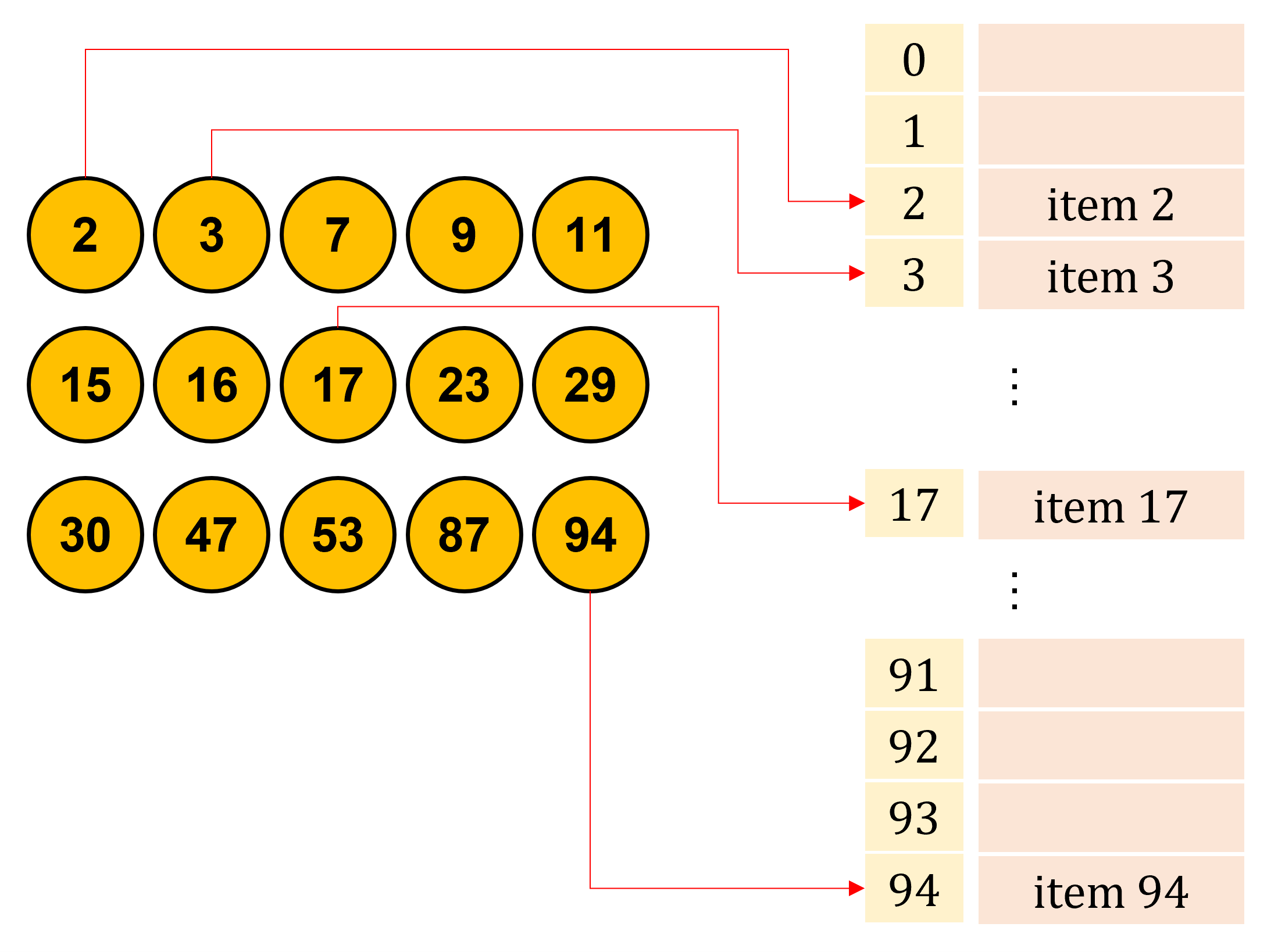
• Waste space

Hash table

• To utilize the space efficiently

  

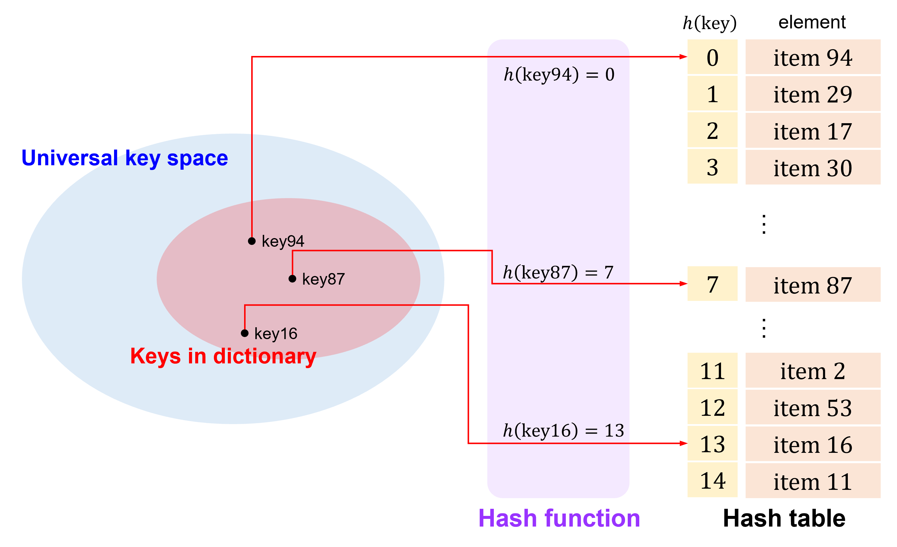
• Assuming the number of keys is \(n\), and the size of table is \(m\). The objective of the hash function is mapping \(n\) possible keys to \(m\) buckets (the size of hash table) so that \(\text{the index of bucket} = h(\text{key})\).

• However, this is very difficult because the size of universal key space is usually \(\gg m\), resulting in the collision, i.e. mapping two different keys to the same bucket (index).

• In this course, we are going to introduce 2 fundamental approaches to create the hash function. For more approaches, you can learn it from the other courses in this campus or the Internet.

---

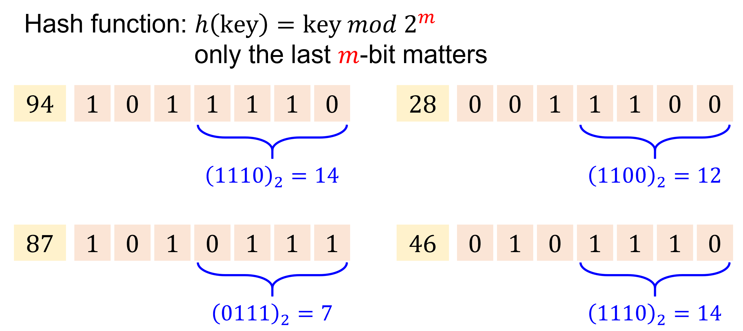
Division method

• Calculate the remainder via modulus: \(h(\text{key}) = \text{key} \ mod \ m\) for \(m\) buckets.

  • Ex: \(m = 16\)

  \[\begin{split} \begin{aligned} h(\text{key94}) &= 94 \ mod \ 16 &= 14, & \ \text{the item of key94 will be put into the} \ 14^{th} \ \text{bucket.} \\ h(\text{key28}) &= 28 \ mod \ 16 &= 12, & \ \text{the item of key28 will be put into the} \ 12^{th} \ \text{bucket.} \\ h(\text{key87}) &= 87 \ mod \ 16 &= 7, & \ \text{the item of key87 will be put into the} \ 7^{th} \ \text{bucket.} \\ h(\text{key46}) &= 46 \ mod \ 16 &= 14, & \ \text{the item of key46 will be put into the} \ {\color{#FFFF00}{14^{th}}} \ \text{bucket.} \\ \end{aligned} \end{split}\]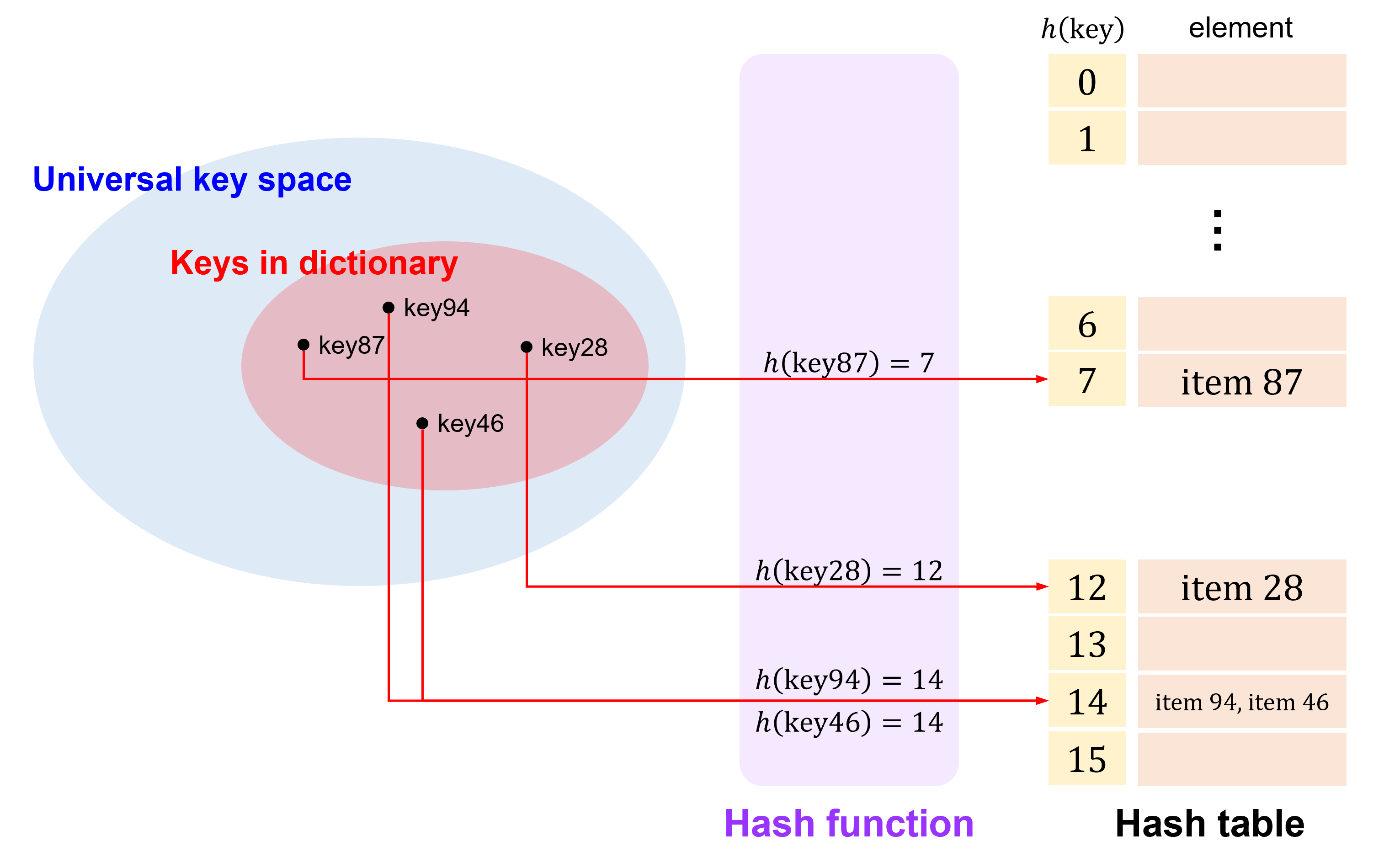
  

  • Pros: Quick

  • Cons: It is not easy to choose an optimal \(m\) (because we never know the range of data).

  

---

Multiplication method

• Because we never know the range or the distribution of key, it is difficult to choose an optimal \(m\) for general cases.

• Another way:

  1. Assuming the size of hash table \({\color{#FFFF00}{m}} = 2^p\)

  2. Choose a constant \({\color{#FFFF00}{A}} \text{, where} \ 0 < A < 1\)

  3. For a key: \(\color{#FFFF00}{K}\), multiply \(\color{#FFFF00}{K}\) by \(\color{#FFFF00}{A}\), get \(\color{#FFFF00}{KA}\)

  4. Extract the fractional part \(\color{#FFFF00}{f}\) of \(\color{#FFFF00}{KA}\), \(f = KA - \lfloor KA \rfloor\)

  5. Multiply \(\color{#FFFF00}{f}\) by \(\color{#FFFF00}{m}\), get \(\color{#FFFF00}{mf}\)

  6. \(h(\text{key}) = \lfloor mf \rfloor\)

• Example:

  \(m = 2^4, \ A = \frac{15}{32}\)

  \(K \ (\text{decimal number})\)	\(K \ (\text{binary number})\)	\(KA\)	\(f\)	\(mf\)	\(h(\text{key})\)
  \(94\)	\((1011110)_2\)	\(\frac{1410}{32} = 44 + \frac{1}{16}\)	\((0.00010)_2\)	\((0001.0)_2\)	\(1\)
  \(28\)	\((0011100)_2\)	\(\frac{420}{32} = 13 + \frac{1}{8}\)	\((0.00100)_2\)	\((0010.0)_2\)	\(2\)
  \(87\)	\((1010111)_2\)	\(\frac{1305}{32} = 40 + \frac{1}{2} + \frac{1}{4} + \frac{1}{32}\)	\((0.11001)_2\)	\((1100.1)_2\)	\(12\)
  \(46\)	\((0101110)_2\)	\(\frac{690}{32} = 21 + \frac{1}{2} + \frac{1}{16}\)	\((0.10010)_2\)	\((1001.0)_2\)	\(9\)

• How to choose \(A\)?

  • Use golden ratio: \(\frac{\sqrt{5}-1}{2}\)

• For more information, please refer to:

  • Second Round