13. Introduction to NumPy and Matplotlib II

• Please refer to here for the data in this lecture.

Last time

• Python package: NumPy

• Python package: Matplotlib

Today

• More on Python package: NumPy
• More on Python package: Matplotlib
• The colorbar of Matplotlib

More on Python package: NumPy

2D array

• Can be directly ceated by list or other methods

import numpy as np
import matplotlib.pyplot as plt

tmp = [
    [1, 3, 5, 7, 9],
    [2, 4, 6, 8, 10],
]
a = np.array(tmp)

print("a:", a)
print("dtype:", a.dtype)
print("shape:", a.shape)

a: [[ 1  3  5  7  9]
 [ 2  4  6  8 10]]
dtype: int32
shape: (2, 5)

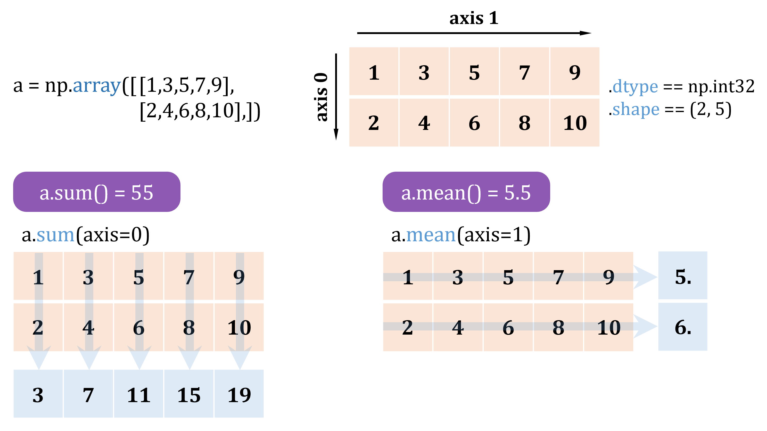
print("a.sum():", a.sum())
print("a.mean():", a.mean())
print("a.sum(axis=0):", a.sum(axis=0))
print("a.mean(axis=1):", a.mean(axis=1))

a.sum(): 55
a.mean(): 5.5
a.sum(axis=0): [ 3  7 11 15 19]
a.mean(axis=1): [5. 6.]

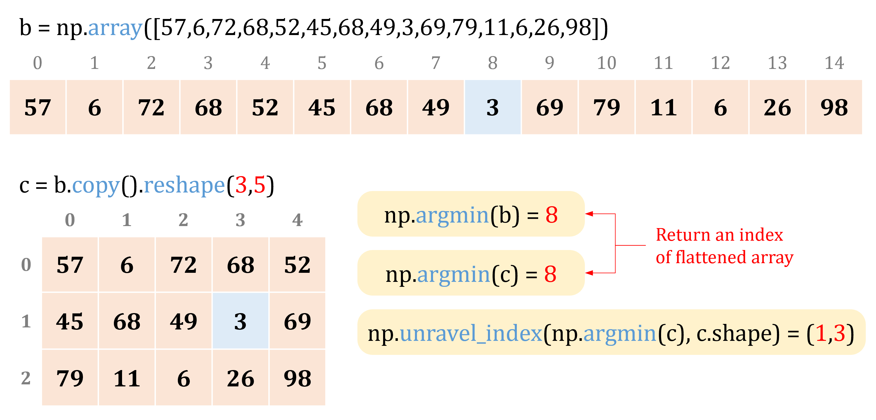
np.unravel_index

• Converts a flat index or array of flat indices into a tuple of coordinate arrays.

• Syntax

  np.unravel_index(indices, shape, order='C')
  

# b = np.random.randint(0, 99, size=(15,))
b = np.array(
    [57, 6, 72, 68, 52, 45, 68, 49, 3, 69, 79, 11, 6, 26, 98]
)
c = b.copy().reshape(3,5)

print("b:", b)
print("c:\n", c)

b: [57  6 72 68 52 45 68 49  3 69 79 11  6 26 98]
c:
 [[57  6 72 68 52]
 [45 68 49  3 69]
 [79 11  6 26 98]]

print("Index of b.min():", np.argmin(b))
print("Index of c.min():", np.argmin(c))    # Return an index of flattened array
print("="*50)
print("Index of c.min():", np.unravel_index(np.argmin(c), c.shape))

Index of b.min(): 8
Index of c.min(): 8
==================================================
Index of c.min(): (1, 3)

---

# Array reshape
print("c:\n", c)
print("c.ravel():\n", c.ravel())
print("c.reshape(-1):\n", c.reshape(-1))
print("c.flatten():\n", c.flatten())
# add new axis
print("c[np.newaxis,:].shape:", c[np.newaxis,:].shape)
print("c[None,:].shape:", c[None,:].shape)
print("c.reshape(1,3,5):", c.reshape(1,3,5).shape)
print("c[:,np.newaxis].shape:", c[:,np.newaxis].shape)
print("c[:,:,np.newaxis].shape:", c[:,:,np.newaxis].shape)

c:
 [[57  6 72 68 52]
 [45 68 49  3 69]
 [79 11  6 26 98]]
c.ravel():
 [57  6 72 68 52 45 68 49  3 69 79 11  6 26 98]
c.reshape(-1):
 [57  6 72 68 52 45 68 49  3 69 79 11  6 26 98]
c.flatten():
 [57  6 72 68 52 45 68 49  3 69 79 11  6 26 98]
c[np.newaxis,:].shape: (1, 3, 5)
c[None,:].shape: (1, 3, 5)
c.reshape(1,3,5): (1, 3, 5)
c[:,np.newaxis].shape: (3, 1, 5)
c[:,:,np.newaxis].shape: (3, 5, 1)

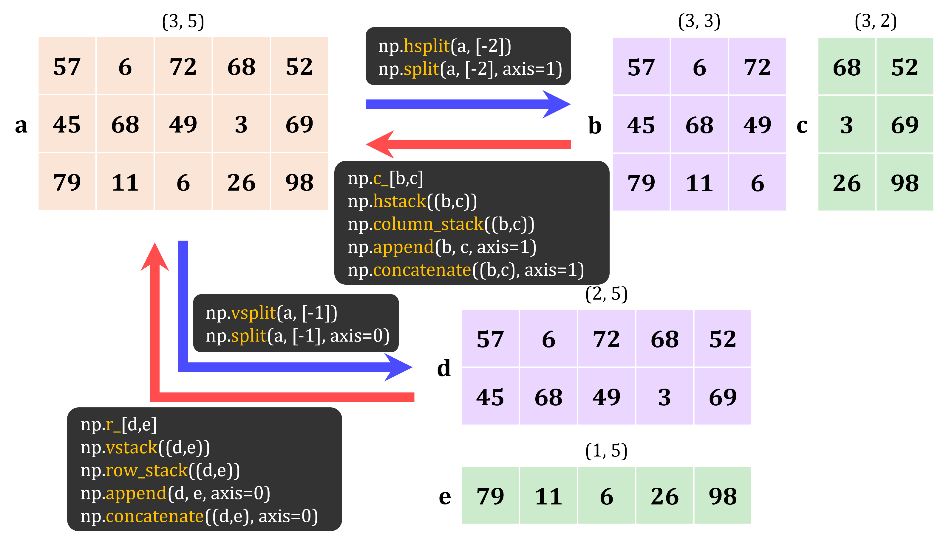
Array combination and seperation

a = np.array(
    [57, 6, 72, 68, 52, 45, 68, 49, 3, 69, 79, 11, 6, 26, 98]
).reshape(3,5)

# horizontal split
# b, c = np.hsplit(a, [-2])
b, c = np.split(a, [-2], axis=1)

print("a:\n", a)
print("b:\n", b)
print("c:\n", c)

# vertical split
# d, e = np.vsplit(a, [-1])
d, e = np.split(a, [-1], axis=0)

print("d:\n", d)
print("e:\n", e)

a:
 [[57  6 72 68 52]
 [45 68 49  3 69]
 [79 11  6 26 98]]
b:
 [[57  6 72]
 [45 68 49]
 [79 11  6]]
c:
 [[68 52]
 [ 3 69]
 [26 98]]
d:
 [[57  6 72 68 52]
 [45 68 49  3 69]]
e:
 [[79 11  6 26 98]]

print("np.c_[b,c]:\n", np.c_[b,c])
print("np.hstack((b,c)):\n", np.hstack((b,c)))
print("np.column_stack((b,c)):\n", np.column_stack((b,c)))
print("np.append(b,c,axis=1):\n", np.append(b,c,axis=1))
print("np.concatenate((b,c),axis=1):\n", np.concatenate((b,c),axis=1))

np.c_[b,c]:
 [[57  6 72 68 52]
 [45 68 49  3 69]
 [79 11  6 26 98]]
np.hstack((b,c)):
 [[57  6 72 68 52]
 [45 68 49  3 69]
 [79 11  6 26 98]]
np.column_stack((b,c)):
 [[57  6 72 68 52]
 [45 68 49  3 69]
 [79 11  6 26 98]]
np.append(b,c,axis=1):
 [[57  6 72 68 52]
 [45 68 49  3 69]
 [79 11  6 26 98]]
np.concatenate((b,c),axis=1):
 [[57  6 72 68 52]
 [45 68 49  3 69]
 [79 11  6 26 98]]

print("np.r_[d,e]:\n", np.r_[d,e])
print("np.vstack((d,e)):\n", np.vstack((d,e)))
print("np.row_stack((d,e)):\n", np.row_stack((d,e)))
print("np.append(d,e,axis=0):\n", np.append(d,e,axis=0))
print("np.concatenate((d,e),axis=0):\n", np.concatenate((d,e),axis=0))

np.r_[d,e]:
 [[57  6 72 68 52]
 [45 68 49  3 69]
 [79 11  6 26 98]]
np.vstack((d,e)):
 [[57  6 72 68 52]
 [45 68 49  3 69]
 [79 11  6 26 98]]
np.row_stack((d,e)):
 [[57  6 72 68 52]
 [45 68 49  3 69]
 [79 11  6 26 98]]
np.append(d,e,axis=0):
 [[57  6 72 68 52]
 [45 68 49  3 69]
 [79 11  6 26 98]]
np.concatenate((d,e),axis=0):
 [[57  6 72 68 52]
 [45 68 49  3 69]
 [79 11  6 26 98]]

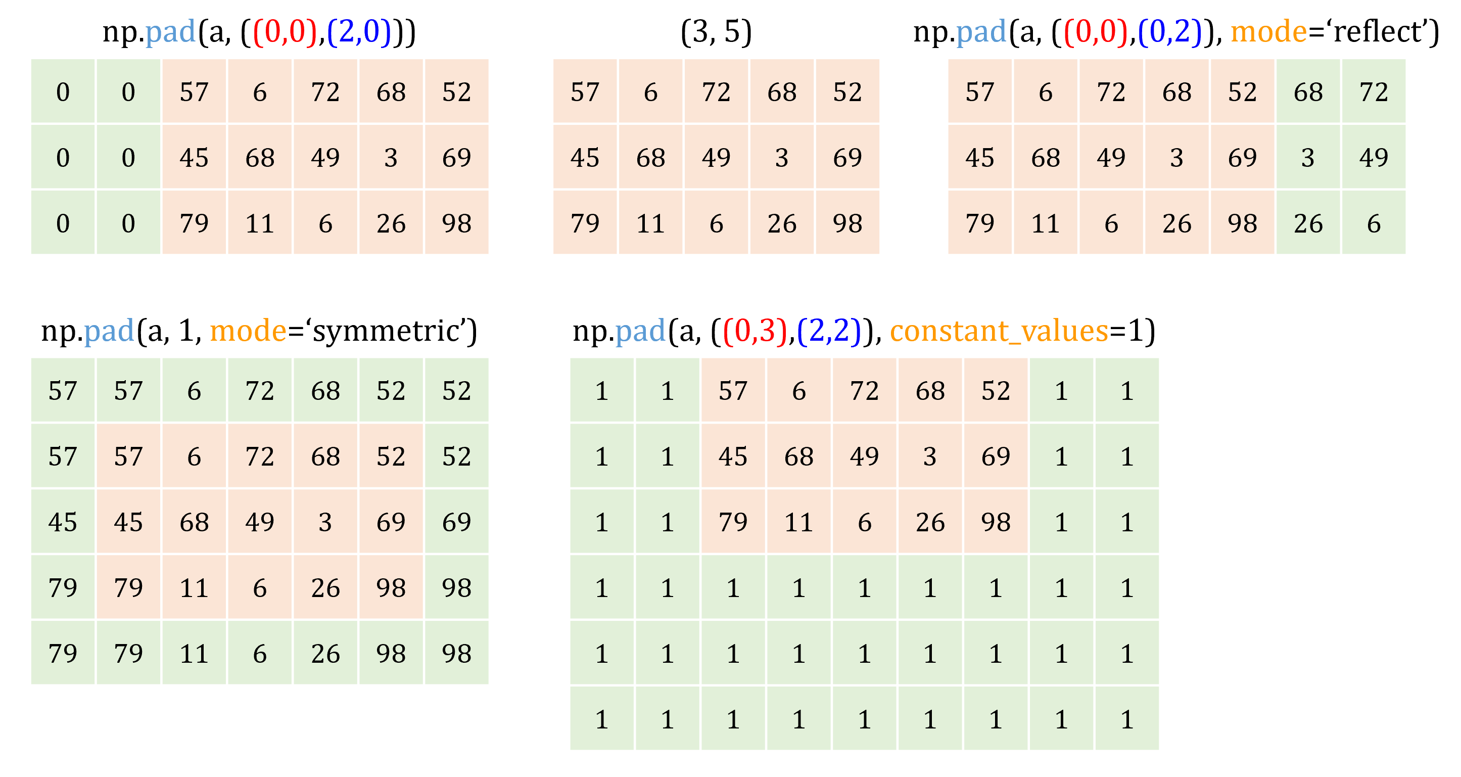
Array padding

• Pad an array

a = np.array(
    [57, 6, 72, 68, 52, 45, 68, 49, 3, 69, 79, 11, 6, 26, 98]
).reshape(3,5)

print("np.pad(a, ((0,0),(2,0))):\n", np.pad(a, ((0,0),(2,0))))
print("np.pad(a, ((0,0),(0,2)), mode='reflect'):\n", np.pad(a, ((0,0),(0,2)), mode='reflect'))
print("np.pad(a, 1, mode='symmetric'):\n", np.pad(a, 1, mode='symmetric'))
print("np.pad(a, ((0,3),(2,2)), constant_values=1):\n", np.pad(a, ((0,3),(2,2)), constant_values=1))

np.pad(a, ((0,0),(2,0))):
 [[ 0  0 57  6 72 68 52]
 [ 0  0 45 68 49  3 69]
 [ 0  0 79 11  6 26 98]]
np.pad(a, ((0,0),(0,2)), mode='reflect'):
 [[57  6 72 68 52 68 72]
 [45 68 49  3 69  3 49]
 [79 11  6 26 98 26  6]]
np.pad(a, 1, mode='symmetric'):
 [[57 57  6 72 68 52 52]
 [57 57  6 72 68 52 52]
 [45 45 68 49  3 69 69]
 [79 79 11  6 26 98 98]
 [79 79 11  6 26 98 98]]
np.pad(a, ((0,3),(2,2)), constant_values=1):
 [[ 1  1 57  6 72 68 52  1  1]
 [ 1  1 45 68 49  3 69  1  1]
 [ 1  1 79 11  6 26 98  1  1]
 [ 1  1  1  1  1  1  1  1  1]
 [ 1  1  1  1  1  1  1  1  1]
 [ 1  1  1  1  1  1  1  1  1]]

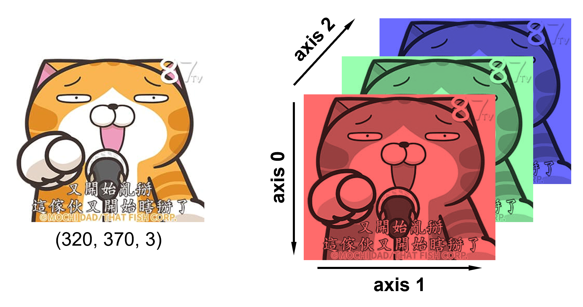
3D array or n-dimensional array

---

More on Python package: Matplotlib

Types of plotting in Matplotlib

• Line plot

• Shaded plot

• Scatter plot

• Boxplot

• Histogram

---

• Heatmap

• Contour map

• Stream plot (To display 2D vector fields)

• Imshow

Supplement: Grid control

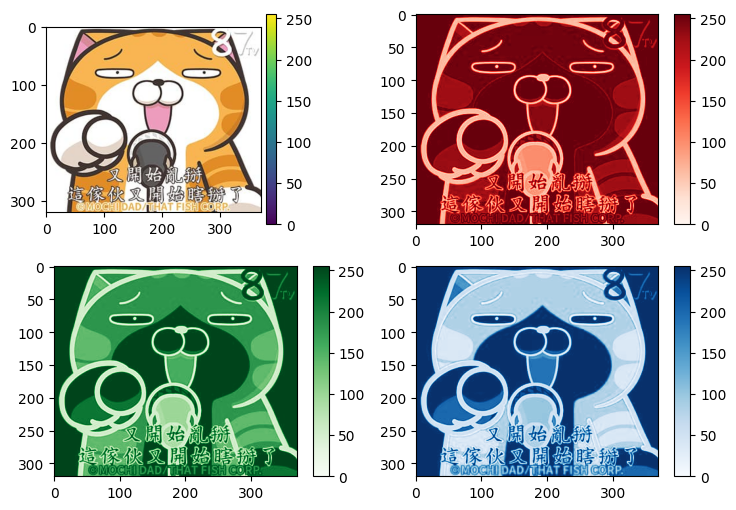
Imshow

• Display data as an image, i.e., on a 2D regular raster.

• Syntax

  Axes.imshow(X, cmap=None, norm=None, *, aspect=None, interpolation=None, alpha=None, 
              vmin=None, vmax=None, origin=None, extent=None, interpolation_stage=None, 
              filternorm=True, filterrad=4.0, resample=None, url=None, data=None, **kwargs)
  

• Documentation

• Choosing Colormaps

import numpy as np
import matplotlib.pyplot as plt

img = np.load(".//data//arr3d.npy")

fig = plt.figure(1, figsize=(10,4), dpi=100)
ax1 = fig.add_subplot(141)
ax1.imshow(img)
ax1.axis("off")
ax2 = fig.add_subplot(142)
ax2.imshow(img[:,:,0], cmap="Reds")
ax2.axis("off")
ax3 = fig.add_subplot(143)
ax3.imshow(img[:,:,1], cmap='Greens')
ax3.axis("off")
ax4 = fig.add_subplot(144)
ax4.imshow(img[:,:,2], cmap='Blues')
ax4.axis("off")

plt.show()

fig, axes = plt.subplots(1, 4, dpi=100, figsize=(10,4))

axes[0].imshow(img)
axes[0].axis("off")

axes[1].imshow(img[:,:,0], cmap="Reds")
axes[1].axis("off")

axes[2].imshow(img[:,:,1], cmap='Greens')
axes[2].axis("off")

axes[3].imshow(img[:,:,2], cmap='Blues')
axes[3].axis("off")

plt.show()

fig, axes = plt.subplots(1, 4, dpi=100, figsize=(10,4))

style = ["Reds", "Greens", "Blues"]

for i in range(len(axes)):
    if i == 0:
        axes[i].imshow(img)
    else:
        axes[i].imshow(img[:,:,i-1], cmap=style[i-1])
    axes[i].axis("off")

plt.show()

fig, axes = plt.subplots(2, 2, dpi=100, figsize=(5,4))

axes[0,0].imshow(img)
axes[0,0].axis("off")

axes[0,1].imshow(img[:,:,0], cmap="Reds")
axes[0,1].axis("off")

axes[1,0].imshow(img[:,:,1], cmap='Greens')
axes[1,0].axis("off")

axes[1,1].imshow(img[:,:,2], cmap='Blues')
axes[1,1].axis("off")

plt.show()

---

Exercise 13.1: Image

• Please write a program that plots below’s figure.

• Your data is here (exercise1.npy)

  img = np.load(".//data//exercise1.npy")
  

• How to generate graylevel image?

\[ Y = 0.299 * R + 0.587 * G + 0.114 * B \]

---

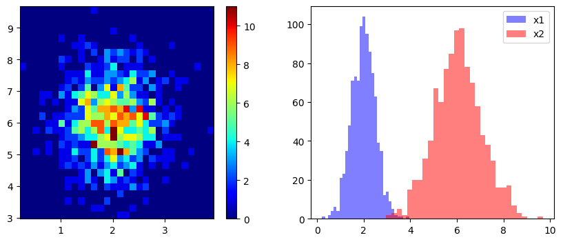
2D histogram

• Make a 2D histogram plot.

• Syntax

  Axes.hist2d(x, y, bins=10, range=None, density=False, weights=None, cmin=None, cmax=None, *, data=None, **kwargs)
  

• Documentation

---

• Example 1: Normal distribution

\[ f(x;\mu, \sigma) = \dfrac{1}{\sigma \sqrt{2\pi}} e^{-\frac{1}{2} \left(\frac{x-\mu}{\sigma}\right)^2} \]

x1 = np.random.normal(loc=2., scale=0.5, size=1000)
x2 = np.random.normal(loc=6., scale=1., size=1000)

fig = plt.figure(figsize=(10, 4))
ax1 = fig.add_subplot(121)
h = ax1.hist2d(x1, x2, bins=30, cmap='jet')
# plt.colorbar(h[3], ax=ax1)
cbar = fig.colorbar(h[3])

ax2 = fig.add_subplot(122)
h = ax2.hist(x1, bins=30, facecolor='blue', alpha=0.5, label='x1')
h = ax2.hist(x2, bins=30, facecolor='red', alpha=0.5, label='x2')
ax2.legend()
plt.show()

Contour map

• Plot contour lines.

• Syntax

  Axes.contour([X, Y,] Z, [levels,] alpha, cmap, linewidths, linestyles, **kwargs)
  Axes.contourf([X, Y,] Z, [levels,] alpha, cmap, linewidths, linestyles, **kwargs)
  

• Documentation

---

• Example: Himmelblau’s function

\[ \begin{equation} f(x,y) = (x^{2}+y-11)^{2} + (x+y^{2}-7)^{2} \end{equation} \]

• Four identical local minimum @\((3.00,2.00),(−2.81,3.13),(−3.80,−3.28),(3.58,−1.85)\)

# Two ways to compute 2D function

# 1. Use np.meshgrid
x = np.linspace(-5, 5, 501)    # Create a 1D array, shape: (501,)
y = np.linspace(-5, 5, 501)    # Create a 1D array, shape: (501,)
xx ,yy = np.meshgrid(x, y)     # Create two 2D arrays, shape: (501, 501)
f1 = (xx**2 + yy - 11)**2 + (xx + yy**2 -7)**2
print("x.shape:", x.shape)
print("y.shape:", y.shape)
print("="*60)

# 2. Use broadcasting
x = np.linspace(-5, 5, 501).reshape(1, -1)    # Create a 1D array then reshape into 2D, shape: (1, 501)
y = np.linspace(-5, 5, 501).reshape(-1, 1)    # Create a 1D array then reshape into 2D, shape: (501, 1)
f2 = (x**2 + y - 11)**2 + (x + y**2 -7)**2
print("x.shape:", x.shape)
print("y.shape:", y.shape)


# Verify f1 and f2
print("Is f1 equal to f2?\n", np.array_equal(f1, f2))

x.shape: (501,)
y.shape: (501,)
============================================================
x.shape: (1, 501)
y.shape: (501, 1)
Is f1 equal to f2?
 True

fig = plt.figure(figsize=(14, 4))

ax1 = fig.add_subplot(121)
im1 = ax1.contour(f2, cmap='brg', levels=20, extent=[-5, 5, -5, 5])
ax1.clabel(im1, inline=True, fontsize=8)
# Use logarithm to enhance the contrast
ax2 = fig.add_subplot(122)
im2 = ax2.contour(xx, yy, np.log(1+f2), cmap='cividis', levels=20, extent=[-5, 5, -5, 5])
ax2.clabel(im2, inline=True, fontsize=8)

plt.show()

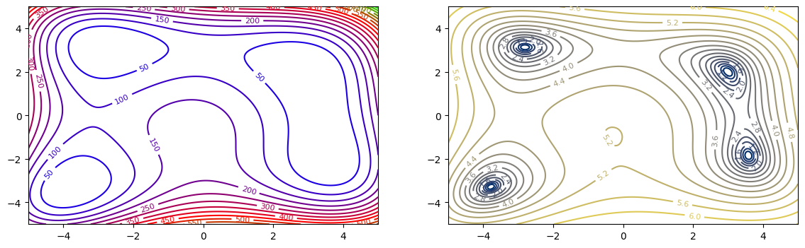
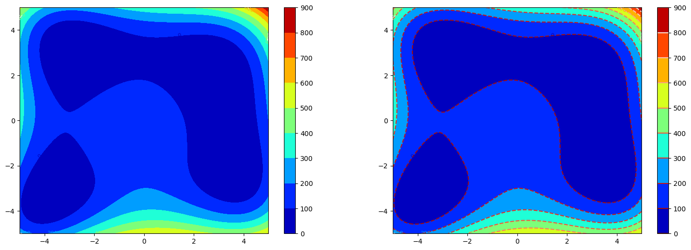
fig = plt.figure(figsize=(18, 6))

# contourf
ax1 = fig.add_subplot(121)
im1 = ax1.contourf(f2, cmap='jet', levels=10, extent=[-5, 5, -5, 5])
ax1.clabel(im1, levels=im1.levels[::2], inline=True, fontsize=8)
cbar = fig.colorbar(im1)

# Use logarithm to enhance the contrast
ax2 = fig.add_subplot(122)
im2 = ax2.contourf(f2, cmap='jet', levels=10, extent=[-5, 5, -5, 5])
ax2.clabel(im2, levels=im2.levels[::2], inline=True, fontsize=8)
# Add contour lines
im3 = ax2.contour(f2, cmap='Reds_r', levels=im2.levels, linestyles='dashed', extent=[-5, 5, -5, 5])
cbar = fig.colorbar(im2)
cbar.add_lines(im3)

plt.show()

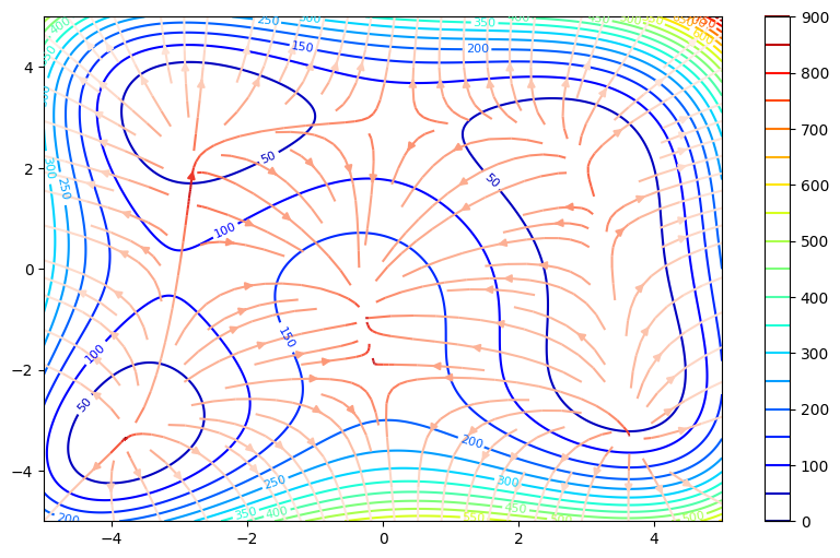
Stream plot

• Draw streamlines of a vector flow.

• Syntax

  Axes.streamplot(x, y, u, v, density=1, linewidth=None, color=None, cmap=None, norm=None, 
                  arrowsize=1, arrowstyle='-|>', minlength=0.1,
                  transform=None, zorder=None, start_points=None, maxlength=4.0, 
                  integration_direction='both', broken_streamlines=True, *, data=None)
  

  • x, y: Evenly spaced strictly increasing arrays to make a grid.

  • u, v: \(x\) and \(y\)-velocities. The number of rows and columns must match the length of y and x, respectively.
    
    

• Documentation

• Example: Himmelblau’s function

\[ \begin{equation} f(x,y) = (x^{2}+y-11)^{2} + (x+y^{2}-7)^{2} \end{equation} \]

\[\begin{split} \begin{align} \nabla f(x,y) &= \dfrac{\partial f}{\partial x} \hat{x} + \dfrac{\partial f}{\partial y} \hat{y} \\ \rightarrow u &= \dfrac{\partial f}{\partial x} = 4 x^3 + 4xy + 2y^2 - 42x - 14 \\ \rightarrow v &= \dfrac{\partial f}{\partial y} = 4 y^3 + 4xy + 2x^2 - 26y - 22 \end{align} \end{split}\]

x = np.linspace(-5, 5, 501).reshape(1, -1)    # Create a 1D array then reshape into 2D, shape: (1, 501)
y = np.linspace(-5, 5, 501).reshape(-1, 1)    # Create a 1D array then reshape into 2D, shape: (501, 1)
f = (x**2 + y - 11)**2 + (x + y**2 -7)**2
u = 4*x**3 + 4*x*y + 2*y**2 - 42*x - 14
v = 4*y**3 + 4*x*x + 2*x**2 - 26*y - 22

fig = plt.figure(figsize=(10, 6))

ax1 = fig.add_subplot(111)
im1 = ax1.contour(f, cmap='jet', levels=20, extent=[-5, 5, -5, 5])
ax1.clabel(im1, inline=True, fontsize=8)

color = np.log(np.hypot(u, v))
# im2 = ax1.streamplot(x, y, u, v, color=color, cmap="terrain")
im2 = ax1.streamplot(x, y, u, v, color=color, cmap="Reds_r")

plt.colorbar(im1, ax=ax1)
plt.show()

---

Exercise 13.2: electric field of point charges

\[ \begin{equation} V_{net} = \sum_{i}{V_{i}} = \dfrac{1}{4\pi\epsilon_{0}} \sum_{i}{\dfrac{q_{i}}{r_{i}}} , \; \text{where} \; r_{i} = \sqrt{(x-x_i)^2 + (y-y_i)^2} \; \text{and} \; (x_i, y_i) \; \text{is the location of point source} \end{equation} \]

\[\begin{split} \begin{aligned} E_{i} = -\nabla V_{i} &= -\dfrac{\partial V_{i}}{\partial x} \hat{x} -\dfrac{\partial V_{i}}{\partial y} \hat{y} \\ \rightarrow E_{i,x} &= -\dfrac{\partial V_{i}}{\partial x}= \dfrac{1}{4\pi\epsilon_{0}} \sum_{i}{\dfrac{q}{r_{i}^{3}} \cdot (x-x_i)}\\ \rightarrow E_{i,y} &= -\dfrac{\partial V_{i}}{\partial y}= \dfrac{1}{4\pi\epsilon_{0}} \sum_{i}{\dfrac{q}{r_{i}^{3}} \cdot (y-y_i)}\\ \rightarrow E_{i} &= \dfrac{1}{4\pi\epsilon_{0}} \sum_{i}{\dfrac{q_i}{r_{i}^{2}}} \end{aligned} \end{split}\]

• Please write a program that plots the electric field of the following conditions:

  1. 1 positive charge \((+q)\) at \((1, 1)\) and 1 negative charge \((-q)\) at \((-1, -1)\)

  2. 2 positive charges \((+q)\) at \((1, 1), (-1,-1)\) and 2 negative charges \((-q)\) at \((1, -1), (-1, 1)\)

---

Exercise 13.2.1

---

Exercise 13.2.2

---

The colorbar of Matplotlib

import numpy as np
import matplotlib.pyplot as plt

img = np.load(".//data//arr3d.npy")

fig = plt.figure(2, figsize=(12,2), dpi=100)
ax1 = fig.add_subplot(141)
im1 = ax1.imshow(img)
cbar = fig.colorbar(im1, ax=ax1, orientation='vertical', pad=0.05)
# cbar = fig.colorbar(im1, ax=ax1, orientation='vertical', shrink=1, aspect=20, pad=0.05)
ax1.axis("off")

ax2 = fig.add_subplot(142)
im2 = ax2.imshow(img[:,:,0], cmap="Reds")
ax2.axis("off")
ax3 = fig.add_subplot(143)
ax3.imshow(img[:,:,1], cmap='Greens')
ax3.axis("off")
ax4 = fig.add_subplot(144)
ax4.imshow(img[:,:,2], cmap='Blues')
ax4.axis("off")

plt.show()

import matplotlib.transforms as mtransforms


def add_right_cax(ax, pad, width):
    axpos = ax.get_position()
    caxpos = mtransforms.Bbox.from_extents(
        axpos.x1 + pad,
        axpos.y0,
        axpos.x1 + pad + width,
        axpos.y1,
    )
    cax = ax.figure.add_axes(caxpos)
    return cax


pad = 0.02
width = 0.02

fig = plt.figure(2, figsize=(8,6), dpi=100)
fig.subplots_adjust(wspace=0.4)

# Subplot 1
ax1 = fig.add_subplot(221)
im1 = ax1.imshow(img)
cbar1 = fig.colorbar(im1, ax=ax1, orientation='vertical', pad=pad)

# Subplot 2
ax2 = fig.add_subplot(222)
im2 = ax2.imshow(img[:,:,0], cmap="Reds")
ax2pos = ax2.get_position()
cax2 = ax2.figure.add_axes(
    mtransforms.Bbox.from_extents(
        ax2pos.x1 + pad,
        ax2pos.y0,
        ax2pos.x1 + pad + width,
        ax2pos.y1,
    )
)
cbar2 = fig.colorbar(im2, cax=cax2)

# Subplot 3
ax3 = fig.add_subplot(223)
im3 = ax3.imshow(img[:,:,1], cmap='Greens')
cax3 = add_right_cax(ax=ax3, pad=pad, width=width)
cbar3 = fig.colorbar(im3, cax=cax3)

# Subplot 4
ax4 = fig.add_subplot(224)
im4 = ax4.imshow(img[:,:,2], cmap='Blues')
cax4 = add_right_cax(ax=ax4, pad=pad, width=width)
cbar4 = fig.colorbar(im4, cax=cax4)

plt.show()

---

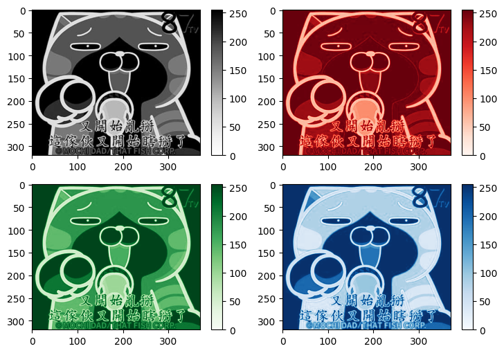
Exercise 13.3:

• Please write a program that plots below’s figure.

• Your data is here (arr3d.npy)

img = np.load(".//data//arr3d.npy")

• How to generate graylevel image?

\[ Y = 0.299 * R + 0.587 * G + 0.114 * B \]

---

---

Don't click this

Exercise 13.2

import numpy as np
import matplotlib.pyplot as plt

def electricPotential(x, y, charges, positions):
    k = (4 * np.pi * 8.854e-12)**(-1)
    V = np.zeros_like(x)
    for charge, position in zip(charges, positions):
        V += k*charge / np.sqrt((x-position[0]) ** 2 + (y-position[1]) ** 2)
    return V

def electricField(x, y, charges, positions):
    k = (4 * np.pi * 8.854e-12)**(-1)
    Ex = np.zeros_like(x)
    Ey = np.zeros_like(x)
    for charge, position in zip(charges, positions):
        den = np.hypot(x-position[0], y-position[1]) ** 3
        Ex += k*charge * (x - position[0]) / den
        Ey += k*charge * (y - position[1]) / den
    return Ex, Ey

x = np.linspace(-3, 3, 200)
y = np.linspace(-3, 3, 200)
xx, yy = np.meshgrid(x, y)

# 1
charges = [-1., 1.]
positions = [(-1, -1), (1, 1)]

V = electricPotential(xx, yy, charges, positions)
Ex, Ey = electricField(xx, yy, charges, positions)

fig = plt.figure(1, figsize=(10, 6), dpi=100)

ax1 = fig.add_subplot(111)
im1 = ax1.imshow(V, origin='lower', cmap='bwr', extent=[-3,3,-3,3])
ax1.grid(True)

color = np.log(np.hypot(Ex, Ey))
im2 = ax1.streamplot(x, y, Ex, Ey, color=color, cmap="terrain")

plt.colorbar(im1, ax=ax1)
plt.show()

Exercise 13.3

import matplotlib.transforms as mtransforms


def add_right_cax(ax, pad, width):
    axpos = ax.get_position()
    caxpos = mtransforms.Bbox.from_extents(
        axpos.x1 + pad,
        axpos.y0,
        axpos.x1 + pad + width,
        axpos.y1,
    )
    cax = ax.figure.add_axes(caxpos)
    return cax

img = np.load(".//data//arr3d.npy")

pad = 0.02
width = 0.02

fig = plt.figure(2, figsize=(8,6), dpi=100)
fig.subplots_adjust(wspace=0.4)
styles = ("Greys", "Reds", "Greens", "Blues")

for i in range(4):
    ax = fig.add_subplot(2, 2, i+1)
    if i == 0:
        im = ax.imshow(
            0.299*img[:,:,0] + 0.587*img[:,:,1] + 0.114*img[:,:,2],
            cmap = styles[i],
        )
    else:
        im = ax.imshow(img[:,:, i-1], cmap=styles[i])
    cax = add_right_cax(ax=ax, pad=pad, width=width)
    cbar = fig.colorbar(im, cax=cax)

plt.show()