12. Introduction to NumPy and Matplotlib I#
Last time#
Searching algorithms
Sorting algorithms
Lambda
Hash table
Today#
Python package: NumPy#
What is NumPy?#
Numerical Python (NumPy) is the fundamental package for scientific computing in Python.
It is an open source library that’s used in every fields of science and engineering. You can say that it is the universal standard for working with numerical data in Python.
Reference:
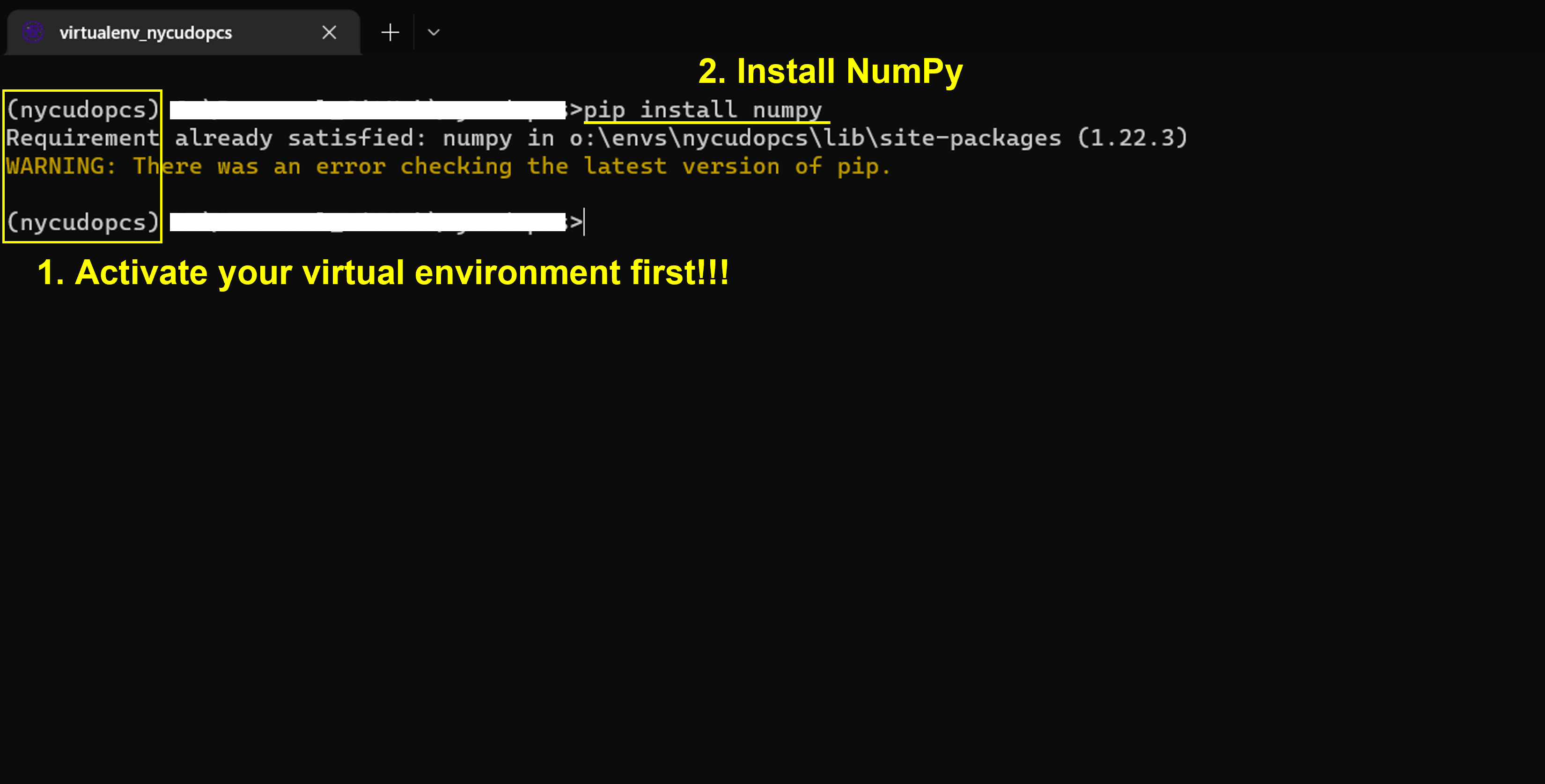
Installing NumPy#
Activate your virtual environment
Install
NumPypip install numpy
Array: numpy.ndarray#
A grid of values with the same data type (can be check via
numpy.ndarray.dtype)Indexed by a tuple of nonnegative integers
Rank: the number of dimensions (can be check via
numpy.ndarray.ndim)Shape: the size of the array along each dimension (can be check via
numpy.ndarray.shape)More array attributes: Refer to here
import numpy as np

a = np.arange(5)

print(a)
print("Type of a:", type(a))
print("Data type of a:", a.dtype)
print("Rank of a:", a.ndim)
print("Shape of a:", a.shape)

print("="*50)

b = np.ones((4,3), dtype=np.float16)

print(b)
print("Type of b:", type(b))
print("Data type of b:", b.dtype)
print("Rank of b:", b.ndim)
print("Shape of b:", b.shape)
[0 1 2 3 4]
Type of a: <class 'numpy.ndarray'>
Data type of a: int32
Rank of a: 1
Shape of a: (5,)
==================================================
[[1. 1. 1.]
 [1. 1. 1.]
 [1. 1. 1.]
 [1. 1. 1.]]
Type of b: <class 'numpy.ndarray'>
Data type of b: float16
Rank of b: 2
Shape of b: (4, 3)
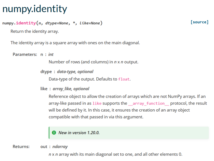
Important skill: read the documentation#
NumPy array vs. Python list#
Example 1: Add two arrays
# list
a = [1, 2, 3, 4, 5]
b = [-5, 3, 2, 0, 8]
print("a + b =", a + b)
print([v1+v2 for v1, v2 in zip(a, b)])
a + b = [1, 2, 3, 4, 5, -5, 3, 2, 0, 8]
[-4, 5, 5, 4, 13]
# numpy array
a = np.array([1, 2, 3, 4, 5])
b = np.array([-5, 3, 2, 0, 8])
print("a + b =", a + b)
a + b = [-4 5 5 4 13]
Example 2: Multiply two arrays element-wisely
# list
a = [1, 2, 3, 4, 5]
b = [-5, 3, 2, 0, 8]
# print("a * b =", a * b)
print([v1*v2 for v1, v2 in zip(a, b)])
[-5, 6, 6, 0, 40]
# numpy array
a = np.array([1, 2, 3, 4, 5])
b = np.array([-5, 3, 2, 0, 8])
print("a * b =", a * b)
a * b = [-5 6 6 0 40]
1D array#
Can be directly ceated by
listor other methods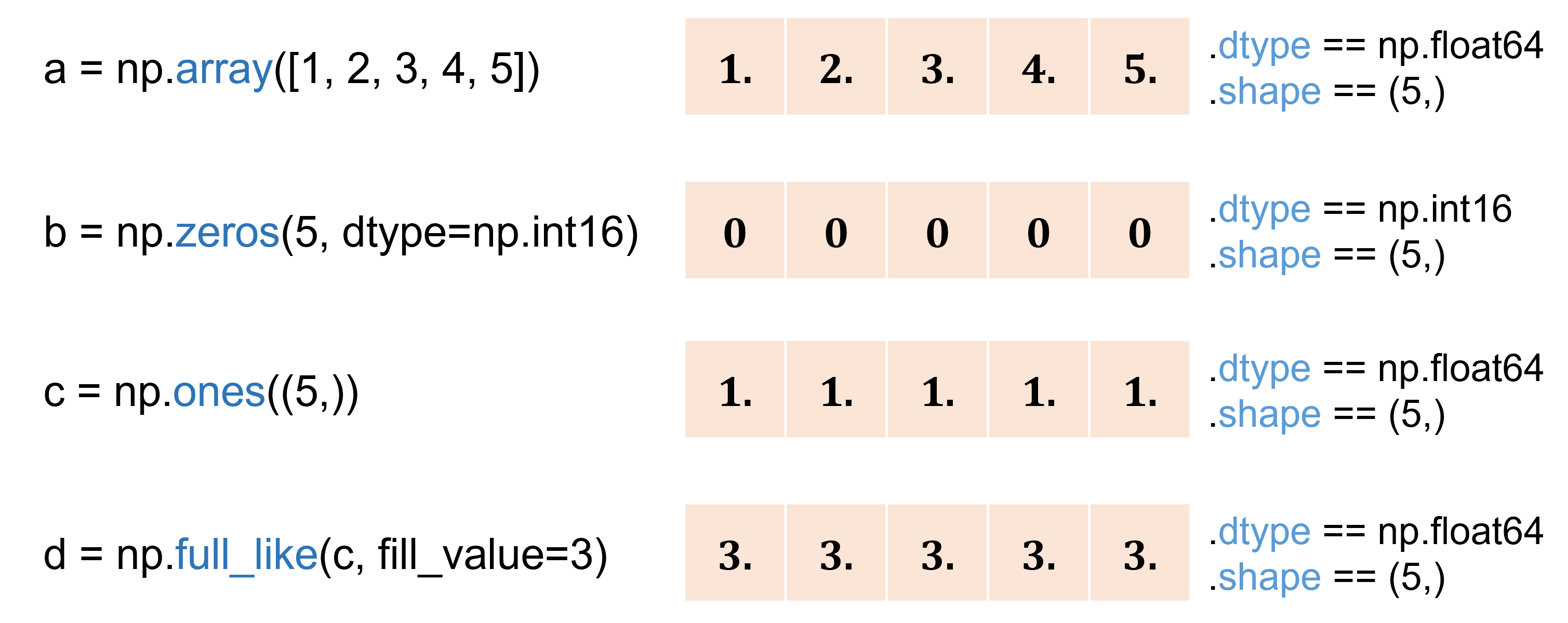
tmp = [1,3,5,7,9]
a = np.array(tmp)
b = np.zeros(5, dtype=np.int16)
c = np.ones((5,))
d = np.full_like(a, fill_value=5)

print("a:", a, "dtype:", a.dtype)
print("b:", b, "dtype:", b.dtype)
print("c:", c, "dtype:", c.dtype)
print("d:", d, "dtype:", d.dtype)
a: [1 3 5 7 9] dtype: int32
b: [0 0 0 0 0] dtype: int16
c: [1. 1. 1. 1. 1.] dtype: float64
d: [5 5 5 5 5] dtype: int32
Create evenly spaced numbers
np.arange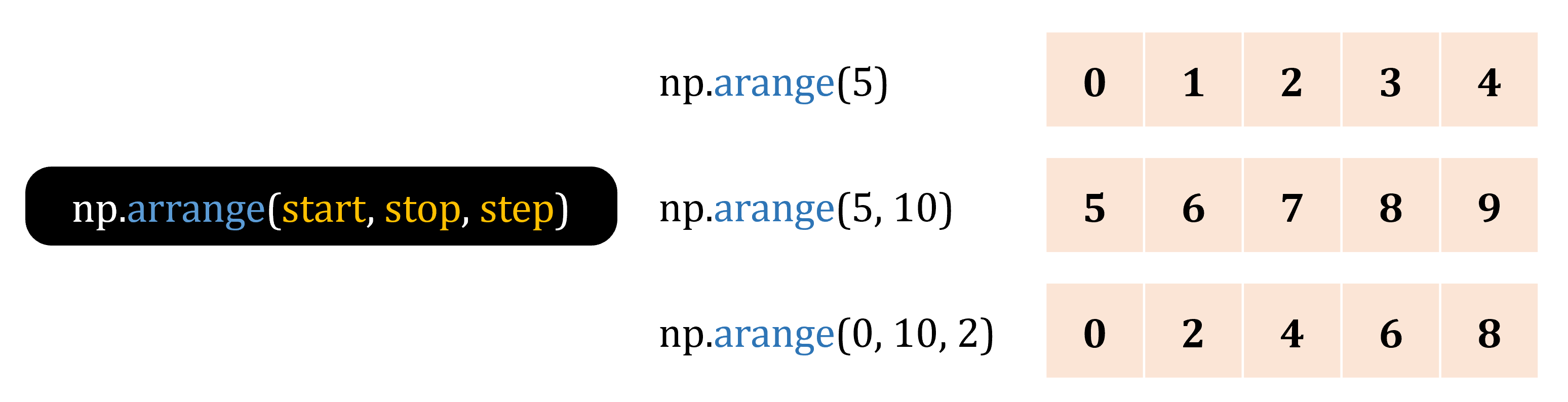
a = np.arange(5)
b = np.arange(5,10)
c = np.arange(0,10,2)

print("a:", a, "dtype:", a.dtype)
print("b:", b, "dtype:", b.dtype)
print("c:", c, "dtype:", c.dtype)
a: [0 1 2 3 4] dtype: int32
b: [5 6 7 8 9] dtype: int32
c: [0 2 4 6 8] dtype: int32
np.linspace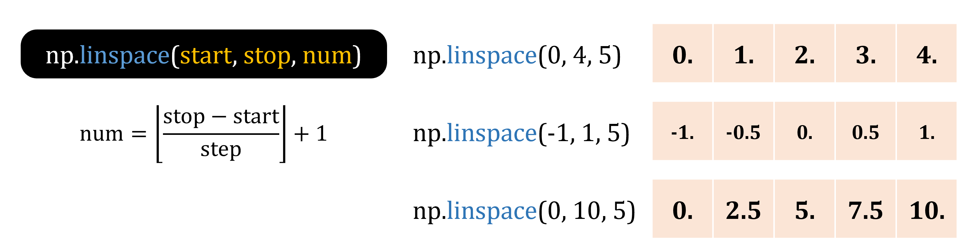
a = np.linspace(0, 4, 5)
b = np.linspace(start=-1, stop=1, num=5)
c = np.linspace(
    start=0,
    stop=10,
    num=5,
)

print("a:", a, "dtype:", a.dtype)
print("b:", b, "dtype:", b.dtype)
print("c:", c, "dtype:", c.dtype)
a: [0. 1. 2. 3. 4.] dtype: float64
b: [-1.  -0.5  0.   0.5  1. ] dtype: float64
c: [ 0.   2.5  5.   7.5 10. ] dtype: float64
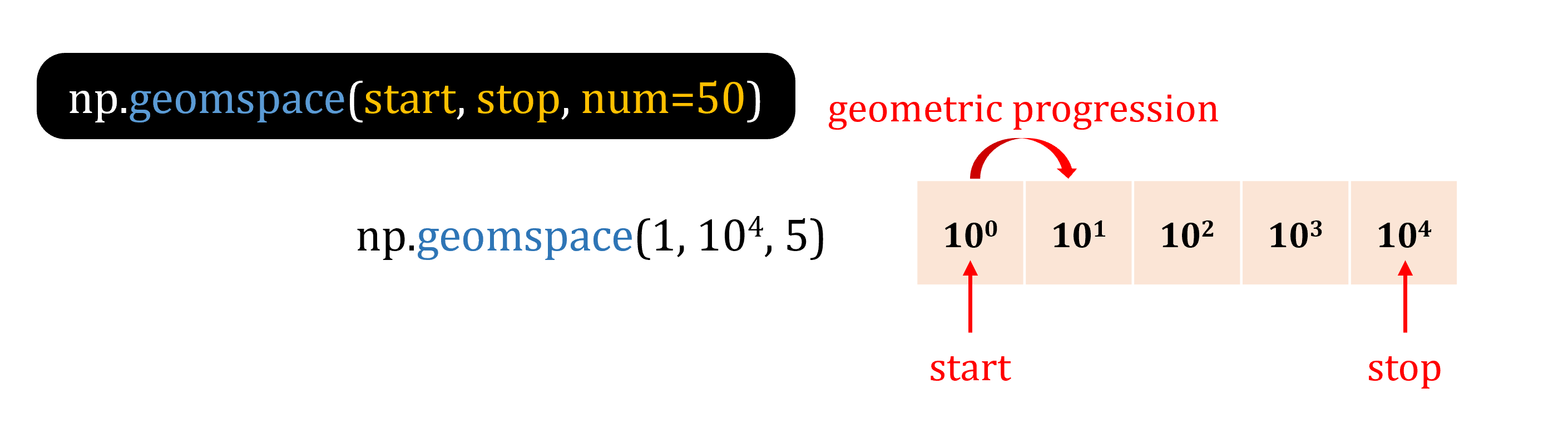
np.logspaceandnp.geomspaceReturn numbers spaced evenly on a log scale.
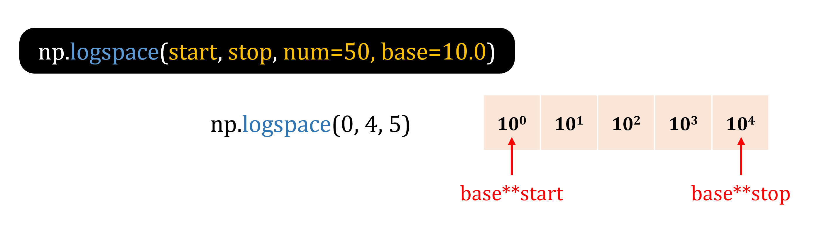
a = np.logspace(start=0, stop=4, num=5, base=10.)
b = np.geomspace(start=1e0, stop=1e4, num=5)

print("a:", a, "dtype:", a.dtype)
print("b:", b, "dtype:", b.dtype)
a: [1.e+00 1.e+01 1.e+02 1.e+03 1.e+04] dtype: float64
b: [1.e+00 1.e+01 1.e+02 1.e+03 1.e+04] dtype: float64
Exercise 12.1#
Please create the following
np.array:
Index |
Array |
|---|---|
1 |
|
2 |
|
3 |
|
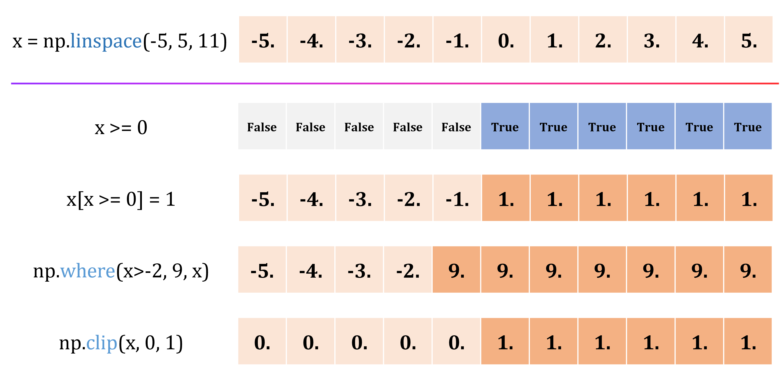
Boolean indexing#
x = np.linspace(-5, 5, 11)

print("x:          ", x)
print("x >= 0:     ", x>=0)

x[x>=3] = 3
print("x[x>=3] = 3:", x)

print("np.where:   ", np.where(x>-2, 9, x))
print("np.clip:    ", np.clip(x, -2, 2))
x:           [-5. -4. -3. -2. -1.  0.  1.  2.  3.  4.  5.]
x >= 0:      [False False False False False  True  True  True  True  True  True]
x[x>=3] = 3: [-5. -4. -3. -2. -1.  0.  1.  2.  3.  3.  3.]
np.where:    [-5. -4. -3. -2.  9.  9.  9.  9.  9.  9.  9.]
np.clip:     [-2. -2. -2. -2. -1.  0.  1.  2.  2.  2.  2.]
Numerical operations on arrays#
Numpy provides a variety of mathematical functions
Trigonometric functions
np.sin,np.cos,np.tan,np.arcsin,np.arccos,np.deg2rad,np.rad2degHyperbolic functions
np.sinh,np.cosh,np.tanh,np.arcsinh,np.arccosh,np.arctanhRounding
np.around,np.floor,np.ceil,np.trunc,np.fixComplex numbers
np.angle,np.real,np.imag,np.conj
Python package: Matplotlib#
What is Matplotlib?#
A popular visualization library, most importantly, it is free and open source (vs. Matlab).
Good for visualizing 1D, 2D (or 3D) data
Support
numpy.ndarrayandlistReference:
Installing matplotlib#
Activate your virtual environment
Install
matplotlibpip install matplotlib
Types of plotting in Matplotlib#
Stream plot (To display 2D vector fields)
And so on…
Supplement: Grid control
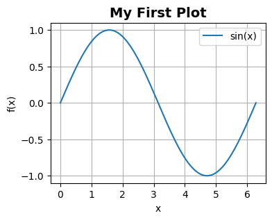
Draw a first plot#
Import module
import matplotlib.pyplot as plt
Imperative syntax
x = np.linspace(0, 2 * np.pi, 200)
y = np.sin(x)

plt.figure(1, figsize=(4,3), dpi=100)
plt.plot(x, y, label="sin(x)")
plt.title("My First Plot", fontsize=14, fontweight='bold')
plt.xlabel("x")
plt.ylabel("f(x)")
plt.grid(True)
plt.legend(loc="best")
plt.show()
Object-oriented syntax
fig = plt.figure(2, figsize=(4,3), dpi=100)
ax = fig.add_subplot(111)
ax.plot(x, y, label="sin(x)")
ax.set_title("My First Plot", fontsize=14, fontweight='bold')
ax.set_xlabel('x')
ax.set_ylabel('f(x)')
ax.legend(loc='best')
ax.grid(True)
# fig.clear()
plt.show()
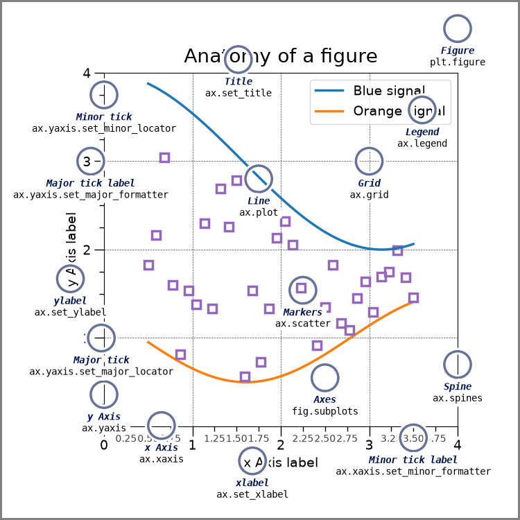
Anatomy of a figure#
Exercise 12.2: Plot a function#
Please write a program that can plot this function \(f(x)\)
Try to meet below’s figure
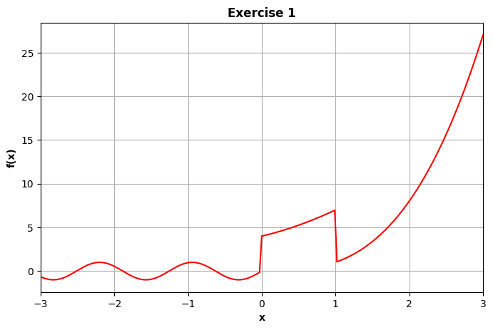
import matplotlib.pyplot as plt
import numpy as np
x = np.linspace(-3, 3, 201)
y = np.where(x < 0, np.sin(5*x), x)
y = np.where(((x >= 0) & (x < 1)), x**2+2*x+4, y)
y = np.where(x >= 1, x**3, y)
fig = plt.figure(figsize=(5, 4), dpi=100, layout="constrained", facecolor="white")
# ax = fig.add_axes((20,3,4,3))
ax = fig.add_subplot(111)
ax.plot(x, y, 'r', label="Exercise 1: f(x)")
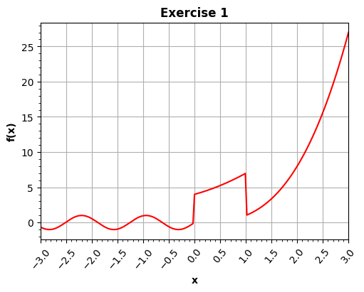
ax.minorticks_on()
ax.xaxis.set_tick_params(rotation=50, labelsize=10)
ax.set_xlim(-3,3)
x_start, x_end = ax.get_xlim()
# ax.xaxis.set_ticks(np.arange(x_start, x_end, 0.5))
ax.xaxis.set_ticks(np.linspace(x_start, x_end, 13))
ax.set_xlabel("x", fontweight='bold')
ax.set_ylabel("f(x)", fontweight='bold')
ax.set_title("Exercise 1", fontweight='bold')
ax.grid(True)
# fig.tight_layout()
# fig.savefig('Exercise1.png')
plt.show()
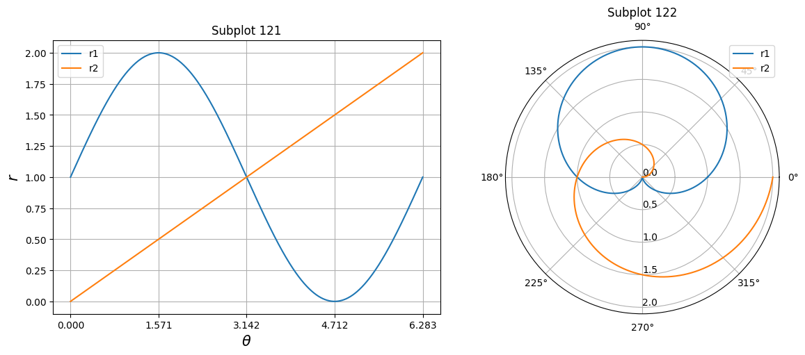
Polar plot#
Plot a curve on a polar axis.
Define \(r\) and \(\theta\) first.
theta = np.linspace(0, 2*np.pi, 1000)
r1 = 1 + np.sin(theta)
r2 = np.linspace(0, 2, 1000)

fig = plt.figure(figsize=(12,5), dpi=100, layout="constrained")

ax1 = fig.add_subplot(121)
ax1.plot(theta, r1, label="r1")
ax1.plot(theta, r2, label="r2")
ax1.set_xticks(np.linspace(0, 2*np.pi, 5))
ax1.grid(True)
ax1.set_title("Subplot 121")
ax1.set_xlabel(r"$\theta$", fontsize=15)
ax1.set_ylabel(r"$r$", fontsize=15)
ax1.legend()

ax2 = fig.add_subplot(122, projection='polar')
ax2.plot(theta, r1, label="r1")
ax2.plot(theta, r2, label="r2")
ax2.set_title("Subplot 122")
ax2.set_rticks(np.linspace(0,2,5))
ax2.set_rlabel_position(-90)
ax2.legend()

# fig.savefig("polar_plot.png", bbox_inches='tight', facecolor='white')

plt.show()
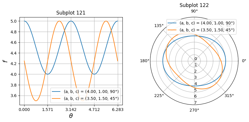
Exercise 12.3: Plot a function#
Please write a program that can plot this function \(f(\theta)\)
Please try different combinations of (a, b, c)
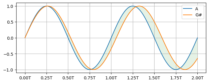
Shaded plot#
Fill the area between two horizontal curves.
freq = 440.0
period = 1 / freq

t = np.linspace(0, 2*period, 100)

c1 = np.sin(2*np.pi*freq*t)
c2 = np.sin(2*np.pi*freq/(2**(1/12))*t)

xticks = []
xticklabels = []
total_ticks = 9

for i in range(total_ticks):
    xticks.append(2*period/8*i)
    xticklabels.append("{:.2f}T".format(i/4))

fig, ax = plt.subplots(1, 1, figsize=(8, 3), dpi=100)
ax.fill_between(t, y1=c1, y2=c2, where=None, color='green', alpha=0.1)
ax.plot(t, c1, label='A')
ax.plot(t, c2, label='G#')
ax.set_xticks(xticks)
ax.set_xticklabels(xticklabels)
# ax.set_xlim(t.max(), 0) # reverse x-axis
ax.legend()
ax.grid(True)
plt.show()
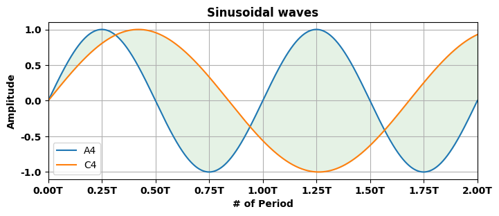
Exercise 12.4: Shaded plot#
Please write a program that plots 2 sinusoidal curves with C4 and A4 frequencies.
Try to meet below’s figure
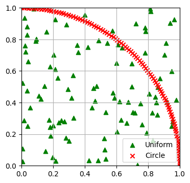
Scatter plot#
A scatter plot of \(y\) vs. \(x\) with varying marker size and/or color.
Syntax
Axes.scatter(x, y, s=None, c=None, marker=None, ...)
num = 100

theta = np.linspace(0, np.pi/2, num)

pdf = np.random.rand(num, num)
cir = np.array([np.cos(theta), np.sin(theta)])

colors = ['green', 'red']
labels = ['Uniform', 'Circle']
markers = ['^', 'x']

fig, ax = plt.subplots(1, 1, figsize=(4, 4), dpi=100)

for color, name, marker, data in zip(colors, labels, markers, (pdf, cir)):
    ax.scatter(data[0], data[1], c=color, label=name, marker=marker)

ax.set_xlim([0,1])
ax.set_ylim([0,1])
ax.legend()
ax.grid(True)
plt.show()
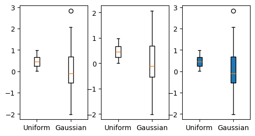
Boxplot#
Draw a box and whisker plot
Syntax
Axes.boxplot(self, x, notch=None, sym=None, vert=None, whis=None,
            positions=None, widths=None, patch_artist=None,
            bootstrap=None, usermedians=None, conf_intervals=None,
            meanline=None, showmeans=None, showcaps=None, showbox=None,
            showfliers=None, labels=None)
num = 100

pdf1 = np.random.rand(num)
pdf2 = np.random.randn(num)

fig = plt.figure(figsize=(6, 3))

ax1 = fig.add_subplot(131)
ax1.boxplot([pdf1, pdf2], meanline=True, showfliers=True)
ax1.set_xticklabels(["Uniform", "Gaussian"])

ax2 = fig.add_subplot(132)
ax2.boxplot([pdf1, pdf2], meanline=True, showfliers=False)
ax2.set_xticklabels(["Uniform", "Gaussian"])

ax3 = fig.add_subplot(133)
ax3.boxplot([pdf1, pdf2], patch_artist=True, meanline=True, showfliers=True)
ax3.set_xticklabels(["Uniform", "Gaussian"])

plt.show()
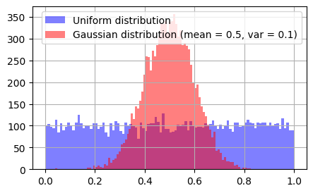
Histogram#
Compute and plot a histogram
Syntax
Axes.hist(x, bins=None, range=None, density=False, weights=None,
        cumulative=False, bottom=None, histtype='bar', align='mid',
        orientation='vertical', rwidth=None, log=False, color=None,
        label=None, stacked=False, *, data=None, **kwargs)
num = 10000
rwidth = 1
nBins = 100
meanGaus, varGaus = 0.5, 0.1

pdf1 = np.random.rand(num)
pdf2 = varGaus*np.random.randn(num) + meanGaus

fig = plt.figure(figsize=(5,3), dpi=100)
ax = fig.add_subplot(111)

n1, bins1, patches1 = ax.hist(
    pdf1,
    bins=nBins,
    rwidth=rwidth,
    facecolor='blue',
    alpha=0.5,
    align='mid',
    label="Uniform distribution"
)
n2, bins2, patches2 = ax.hist(
    pdf2,
    bins=nBins,
    rwidth=rwidth,
    facecolor='red',
    alpha=0.5,
    align='mid',
    label="Gaussian distribution (mean = {}, var = {})".format(meanGaus, varGaus)
)

# ax.set_xlim([0, 1])
# ax.set_ylim([0, np.max(n2)*1.5])
ax.legend(loc="best")
ax.grid(True)

plt.show()
Don't click this
Exercise 12.2
x = np.linspace(-3, 3, 201)
y = np.where(x < 0, np.sin(5*x), x)
y = np.where(((x >= 0) & (x < 1)), x**2+2*x+4, y)
y = np.where(x >= 1, x**3, y)

fig = plt.figure(figsize=(8, 5), dpi=100)
ax = fig.add_subplot()
ax.plot(x, y, 'r', label="Exercise 1: f(x)")
ax.set_xlim(-3,3)
ax.set_xlabel("x", fontweight='bold')
ax.set_ylabel("f(x)", fontweight='bold')
ax.set_title("Exercise 1", fontweight='bold')
plt.grid(True)
# fig.savefig('Exercise1.png', bbox_inches='tight')
plt.show()
Exercise 12.3
theta = np.linspace(0, 2*np.pi, 200)

set1 = (4, 1, np.pi/2)
set2 = (3.5, 1.5, np.pi/4)

f = lambda set: set[0] + set[1]*(np.sin(theta-set[2]))**2

fig = plt.figure(figsize=(10,4), dpi=100)

ax1 = fig.add_subplot(121)
ax1.plot(theta, f(set1), label="(a, b, c) = ({:.2f}, {:.2f}, {:.0f}$\degree$)".format(set1[0], set1[1], set1[2]/np.pi*180))
ax1.plot(theta, f(set2), label="(a, b, c) = ({:.2f}, {:.2f}, {:.0f}$\degree$)".format(set2[0], set2[1], set2[2]/np.pi*180))
ax1.set_xticks(np.linspace(0, 2*np.pi, 5))
ax1.grid(True)
ax1.set_title("Subplot 121")
ax1.set_xlabel(r"$\theta$", fontsize=15)
ax1.set_ylabel(r"$f$", fontsize=15)
ax1.legend()

ax2 = fig.add_subplot(122, projection='polar')
ax2.plot(theta, f(set1), label="(a, b, c) = ({:.2f}, {:.2f}, {:.0f}$\degree$)".format(set1[0], set1[1], set1[2]/np.pi*180))
ax2.plot(theta, f(set2), label="(a, b, c) = ({:.2f}, {:.2f}, {:.0f}$\degree$)".format(set2[0], set2[1], set2[2]/np.pi*180))
ax2.set_title("Subplot 122")
ax2.set_rticks(np.linspace(0,7,8))
ax2.set_rlabel_position(-90)
ax2.legend()

fig.savefig("exercise2.png", bbox_inches='tight', facecolor='white')

plt.show()
Exercise 12.4
freq = 440.0
period = 1 / freq

freq1 = freq/(2**(1/12))**9

t = np.linspace(0, 2*period, 1000)

c1 = np.sin(2*np.pi*freq*t)
c2 = np.sin(2*np.pi*freq1*t)

xticks = []
xticklabels = []
total_ticks = 9

for i in range(total_ticks):
    xticks.append(2*period/8*i)
    xticklabels.append("{:.2f}T".format(i/4))

fig, ax = plt.subplots(1, 1, figsize=(8, 3), dpi=100)
ax.fill_between(t, y1=c1, y2=c2, where=None, color='green', alpha=0.1)
ax.plot(t, c1, label='A4')
ax.plot(t, c2, label='C4')
ax.set_title("Sinusoidal waves", fontweight='bold')
ax.set_ylabel("Amplitude", fontweight='bold')
ax.set_xlabel("# of Period", fontweight='bold')
ax.set_xlim([0, t.max()])
ax.set_xticks(xticks)
ax.set_xticklabels(xticklabels, fontweight='bold')
ax.set_yticks([-1., -0.5, 0., 0.5, 1.])
ax.set_yticklabels([-1., -0.5, 0., 0.5, 1.], fontweight='bold')
ax.legend()
ax.grid(True)
fig.savefig("exercise3.png", bbox_inches='tight', facecolor='white')
plt.show()