14. Data Analysis and More Data Visualization with Python I#
Please refer to here for the data in this lecture.
Last time#
Python package: NumPy
Python package: Matplotlib
Today#
Python package: pandas#
pandasis a Python package providing fast, flexible, and expressive data structures designed to make working with relational or labeled data both easy and intuitive.Reference:
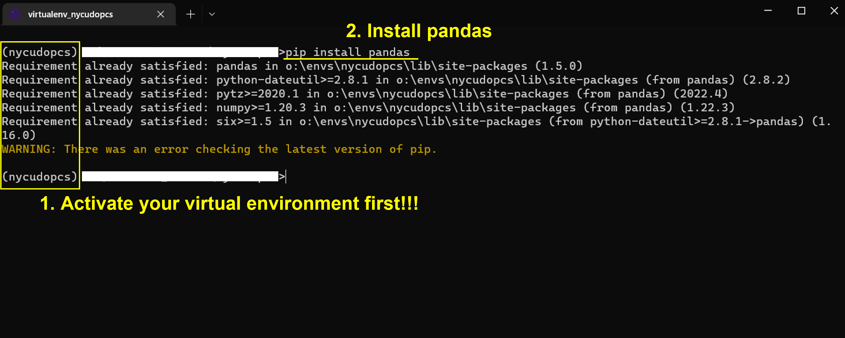
Install pandas#
Activate your virtual environment
Install
pandaspip install pandas
DataFrame and Series#
A
DataFrameis a 2-dimensional data structure that can store data of different types (including characters, integers, floating point values, categorical data and more) in columns.Each column in a
DataFrameis aSeries.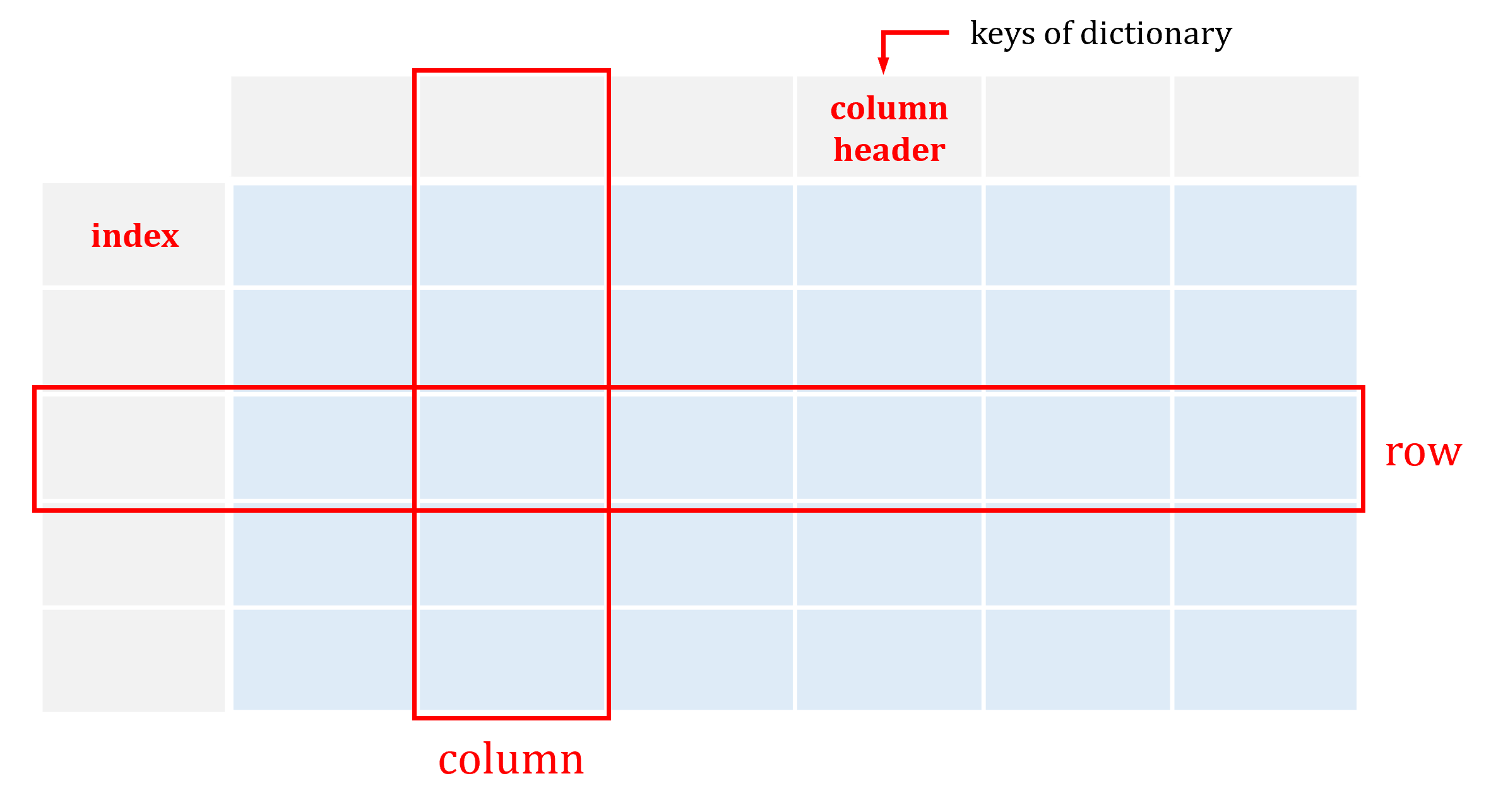
import pandas as pd

df1 = pd.DataFrame({
    "Student ID": ["112514001", "112514002", "112514003", "112514004", "112514005"],
    "Gender": ["Female", "Male", "Third", "Female", "Male"],
    "HW#1": [100, 0, 70, 90, 80],
    "HW#2": [90, 60, 95, 85, 100],
    "HW#3": [100, 75, 80, 100, 60],
})

print(df1)
  Student ID  Gender  HW#1  HW#2  HW#3
0  112514001  Female   100    90   100
1  112514002    Male     0    60    75
2  112514003   Third    70    95    80
3  112514004  Female    90    85   100
4  112514005    Male    80   100    60
print(df1["HW#1"])
0    100
1      0
2     70
3     90
4     80
Name: HW#1, dtype: int64
print(df1.iloc[0])
print("type(df1.iloc[0]):", type(df1.iloc[0]))
Student ID    112514001
Gender           Female
HW#1                100
HW#2                 90
HW#3                100
Name: 0, dtype: object
type(df1.iloc[0]): <class 'pandas.core.series.Series'>
import numpy as np

hw4 = pd.Series(np.random.randint(0, 100, size=(5,)), name="HW#4")

print(hw4)
0    99
1    69
2     1
3    83
4    72
Name: HW#4, dtype: int32
# Add new column
df1["HW#4"] = hw4

print(df1)
  Student ID  Gender  HW#1  HW#2  HW#3  HW#4
0  112514001  Female   100    90   100    99
1  112514002    Male     0    60    75    69
2  112514003   Third    70    95    80     1
3  112514004  Female    90    85   100    83
4  112514005    Male    80   100    60    72
# Add new column from existing columns
df1["Final"] = df1["HW#1"]*0.3 + df1["HW#2"]*0.3 + df1["HW#3"]*0.3 + df1["HW#4"]*0.1

print(df1)
  Student ID  Gender  HW#1  HW#2  HW#3  HW#4  Final
0  112514001  Female   100    90   100    99   96.9
1  112514002    Male     0    60    75    69   47.4
2  112514003   Third    70    95    80     1   73.6
3  112514004  Female    90    85   100    83   90.8
4  112514005    Male    80   100    60    72   79.2
Using
pd.DataFrame.describe()to acquire the basic statistics
# Only for the numerical data
df1.describe()
| HW#1 | HW#2 | HW#3 | HW#4 | Final | |
|---|---|---|---|---|---|
| count | 5.000000 | 5.000000 | 5.000000 | 5.00000 | 5.000000 |
| mean | 68.000000 | 86.000000 | 83.000000 | 64.80000 | 77.580000 |
| std | 39.623226 | 15.572412 | 17.175564 | 37.55263 | 19.218012 |
| min | 0.000000 | 60.000000 | 60.000000 | 1.00000 | 47.400000 |
| 25% | 70.000000 | 85.000000 | 75.000000 | 69.00000 | 73.600000 |
| 50% | 80.000000 | 90.000000 | 80.000000 | 72.00000 | 79.200000 |
| 75% | 90.000000 | 95.000000 | 100.000000 | 83.00000 | 90.800000 |
| max | 100.000000 | 100.000000 | 100.000000 | 99.00000 | 96.900000 |
# Get dtype of each column
print(df1.dtypes)

# Get the shape of the DataFrame
print(df1.shape)
Student ID     object
Gender         object
HW#1            int64
HW#2            int64
HW#3            int64
HW#4            int32
Final         float64
dtype: object
(5, 7)
# data_range

num = 10
dates = pd.date_range("2050-12-25", periods=5, freq="W-THU")
idx = ["1395140{:02d}".format(i+1) for i in range(num)]

df2 = pd.DataFrame(np.random.randint(0, 3, (num, len(dates))), index=idx, columns=dates)

print(df2)
print(df2.index)
print(df2.columns)
           2050-12-29  2051-01-05  2051-01-12  2051-01-19  2051-01-26
139514001           0           1           0           1           0
139514002           2           2           1           2           0
139514003           1           2           0           0           1
139514004           1           1           0           0           0
139514005           0           2           2           1           2
139514006           0           2           2           1           0
139514007           0           2           0           1           1
139514008           1           0           2           0           2
139514009           0           1           2           0           0
139514010           1           2           2           1           2
Index(['139514001', '139514002', '139514003', '139514004', '139514005',
       '139514006', '139514007', '139514008', '139514009', '139514010'],
      dtype='object')
DatetimeIndex(['2050-12-29', '2051-01-05', '2051-01-12', '2051-01-19',
               '2051-01-26'],
              dtype='datetime64[ns]', freq='W-THU')
Read and write tabular data#
Use
DataFrame.to_*for exporting dataUse
pd.read_*for reading dataNote. If you want to read
excelfile viapandas, you need to installopenpyxlbypip install openpyxlfirst.
# exporting df1 as a .csv file

# df1.to_csv("test.csv")
# importing data from a .csv file
batting = pd.read_csv(".//data//data_batting.csv")

print(batting)
        playerID  yearID  stint teamID lgID    G   AB   R   H  2B  ...  RBI  \
0       abadan01    2001      1    OAK   AL    1    1   0   0   0  ...    0
1      abbotje01    2001      1    FLO   NL   28   42   5  11   3  ...    5
2      abbotku01    2001      1    ATL   NL    6    9   0   2   0  ...    0
3      abbotpa01    2001      1    SEA   AL   28    4   0   1   0  ...    0
4      abernbr01    2001      1    TBA   AL   79  304  43  82  17  ...   33
...          ...     ...    ...    ...  ...  ...  ...  ..  ..  ..  ...  ...
20695   zitoba01    2015      1    OAK   AL    3    0   0   0   0  ...    0
20696  zobribe01    2015      1    OAK   AL   67  235  39  63  20  ...   33
20697  zobribe01    2015      2    KCA   AL   59  232  37  66  16  ...   23
20698  zuninmi01    2015      1    SEA   AL  112  350  28  61  11  ...   28
20699   zychto01    2015      1    SEA   AL   13    0   0   0   0  ...    0

       SB  CS  BB   SO  IBB  HBP  SH  SF  GIDP
0       0   0   0    0    0    0   0   0     0
1       0   0   3    7    0    1   0   0     1
2       1   0   0    3    0    0   0   0     0
3       0   0   0    1    0    0   1   0     0
4       8   3  27   35    1    0   3   1     3
...    ..  ..  ..  ...  ...  ...  ..  ..   ...
20695   0   0   0    0    0    0   0   0     0
20696   1   1  33   26    2    0   0   3     5
20697   2   3  29   30    1    1   0   2     3
20698   0   1  21  132    0    5   8   2     6
20699   0   0   0    0    0    0   0   0     0

[20700 rows x 22 columns]
# Only show the first 5 rows
print(batting.head())

# Change n if you need
# print(batting.head(n=7))
    playerID  yearID  stint teamID lgID   G   AB   R   H  2B  ...  RBI  SB  \
0   abadan01    2001      1    OAK   AL   1    1   0   0   0  ...    0   0
1  abbotje01    2001      1    FLO   NL  28   42   5  11   3  ...    5   0
2  abbotku01    2001      1    ATL   NL   6    9   0   2   0  ...    0   1
3  abbotpa01    2001      1    SEA   AL  28    4   0   1   0  ...    0   0
4  abernbr01    2001      1    TBA   AL  79  304  43  82  17  ...   33   8

   CS  BB  SO  IBB  HBP  SH  SF  GIDP
0   0   0   0    0    0   0   0     0
1   0   3   7    0    1   0   0     1
2   0   0   3    0    0   0   0     0
3   0   0   1    0    0   1   0     0
4   3  27  35    1    0   3   1     3

[5 rows x 22 columns]
Filter a subset of a DataFrame#
Example: Extracting the batting statistics of Albert Pujols
# method 1
tmp_list = []

for i in range(batting.shape[0]):
    if batting.iloc[i]["playerID"] == "pujolal01":
        tmp_list.append(batting.iloc[i])

method1 = pd.DataFrame(tmp_list, columns=batting.columns)

print(method1)
        playerID  yearID  stint teamID lgID    G   AB    R    H  2B  ...  RBI  \
972    pujolal01    2001      1    SLN   NL  161  590  112  194  47  ...  130
2302   pujolal01    2002      1    SLN   NL  157  590  118  185  40  ...  127
3616   pujolal01    2003      1    SLN   NL  157  591  137  212  51  ...  124
5010   pujolal01    2004      1    SLN   NL  154  592  133  196  51  ...  123
6314   pujolal01    2005      1    SLN   NL  161  591  129  195  38  ...  117
7674   pujolal01    2006      1    SLN   NL  143  535  119  177  33  ...  137
9065   pujolal01    2007      1    SLN   NL  158  565   99  185  38  ...  103
10451  pujolal01    2008      1    SLN   NL  148  524  100  187  44  ...  116
11836  pujolal01    2009      1    SLN   NL  160  568  124  186  45  ...  135
13197  pujolal01    2010      1    SLN   NL  159  587  115  183  39  ...  118
14578  pujolal01    2011      1    SLN   NL  147  579  105  173  29  ...   99
15995  pujolal01    2012      1    LAA   AL  154  607   85  173  50  ...  105
17411  pujolal01    2013      1    LAA   AL   99  391   49  101  19  ...   64
18825  pujolal01    2014      1    LAA   AL  159  633   89  172  37  ...  105
20297  pujolal01    2015      1    LAA   AL  157  602   85  147  22  ...   95

       SB  CS   BB  SO  IBB  HBP  SH  SF  GIDP
972     1   3   69  93    6    9   1   7    21
2302    2   4   72  69   13    9   0   4    20
3616    5   1   79  65   12   10   0   5    13
5010    5   5   84  52   12    7   0   9    21
6314   16   2   97  65   27    9   0   3    19
7674    7   2   92  50   28    4   0   3    20
9065    2   6   99  58   22    7   0   8    27
10451   7   3  104  54   34    5   0   8    16
11836  16   4  115  64   44    9   0   8    23
13197  14   4  103  76   38    4   0   6    23
14578   9   1   61  58   15    4   0   7    29
15995   8   1   52  76   16    5   0   6    19
17411   1   1   40  55    8    5   0   7    18
18825   5   1   48  71   11    5   0   9    28
20297   5   3   50  72   10    6   0   3    15

[15 rows x 22 columns]
# method 2
method2 = batting[batting["playerID"] == "pujolal01"]

print(method2)
        playerID  yearID  stint teamID lgID    G   AB    R    H  2B  ...  RBI  \
972    pujolal01    2001      1    SLN   NL  161  590  112  194  47  ...  130
2302   pujolal01    2002      1    SLN   NL  157  590  118  185  40  ...  127
3616   pujolal01    2003      1    SLN   NL  157  591  137  212  51  ...  124
5010   pujolal01    2004      1    SLN   NL  154  592  133  196  51  ...  123
6314   pujolal01    2005      1    SLN   NL  161  591  129  195  38  ...  117
7674   pujolal01    2006      1    SLN   NL  143  535  119  177  33  ...  137
9065   pujolal01    2007      1    SLN   NL  158  565   99  185  38  ...  103
10451  pujolal01    2008      1    SLN   NL  148  524  100  187  44  ...  116
11836  pujolal01    2009      1    SLN   NL  160  568  124  186  45  ...  135
13197  pujolal01    2010      1    SLN   NL  159  587  115  183  39  ...  118
14578  pujolal01    2011      1    SLN   NL  147  579  105  173  29  ...   99
15995  pujolal01    2012      1    LAA   AL  154  607   85  173  50  ...  105
17411  pujolal01    2013      1    LAA   AL   99  391   49  101  19  ...   64
18825  pujolal01    2014      1    LAA   AL  159  633   89  172  37  ...  105
20297  pujolal01    2015      1    LAA   AL  157  602   85  147  22  ...   95

       SB  CS   BB  SO  IBB  HBP  SH  SF  GIDP
972     1   3   69  93    6    9   1   7    21
2302    2   4   72  69   13    9   0   4    20
3616    5   1   79  65   12   10   0   5    13
5010    5   5   84  52   12    7   0   9    21
6314   16   2   97  65   27    9   0   3    19
7674    7   2   92  50   28    4   0   3    20
9065    2   6   99  58   22    7   0   8    27
10451   7   3  104  54   34    5   0   8    16
11836  16   4  115  64   44    9   0   8    23
13197  14   4  103  76   38    4   0   6    23
14578   9   1   61  58   15    4   0   7    29
15995   8   1   52  76   16    5   0   6    19
17411   1   1   40  55    8    5   0   7    18
18825   5   1   48  71   11    5   0   9    28
20297   5   3   50  72   10    6   0   3    15

[15 rows x 22 columns]
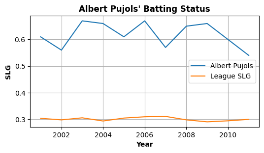
Exercise 14.1: calculate the slugging percentage (SLG)#
Please write a program that calculates the slugging percentage (SLG) of Albert Pujols during his first career in St. Louis Cardinals (2001-2011).
Please also calculate the average SLG of the entire league during 2001-2011.
The definition of SLG is:
Please plot the result:

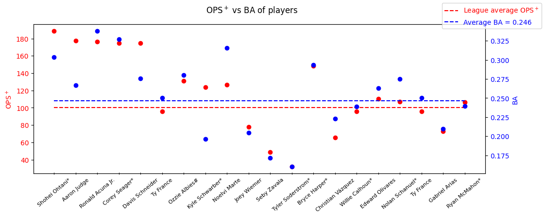
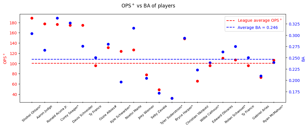
Exercise 14.2: calculate the OPS+#
Please write a program that calculates the On-base Plus Slugging Plus (\(\text{OPS}^+\)) of all players that had played in MLB 2023 seasons.
The definitions of Batting Average (BA), On-based Percentage (OBP), On-based Plus Slugging (OPS), and \(\text{OPS}^+\) are:
Please plot the result:
Style 1
Style 2
Exercise 14.3: calculate the wOBA, wRAA, and wRC#
Please write a program that calculates the weighted on-base average (wOBA), weighted runs above average (wRAA), and weighted Runs Created (wRC) of all player that had played in MLB 2023 season.
The definitions of wOBA, wRAA, and wRC of MLB 2023 are:
Please plot the result:
Style 1

Style 2

Reference#
The data of this lecture is from Baseball Reference, FanGraphs BaseBall, and Kaggle.com.
Don't click this
Exercise 14.1
import numpy as np
import pandas as pd
import matplotlib.pyplot as plt

batting = pd.read_csv(".//data//data_batting.csv")
pujols = batting[batting["playerID"] == "pujolal01"]

data = pujols[pujols["teamID"] == "SLN"][["playerID", "yearID", "teamID", "AB", "H", "2B", "3B", "HR"]]

data["SLG"] = (((data["H"]-data["2B"]-data["3B"]-data["HR"]) + 2*data["2B"] + 3*data["3B"] + 4*data["HR"])/data["AB"]).round(2)

slg_all = []

for i in range(data.shape[0]):
    data_all = batting[batting["yearID"] == (2001+i) ][["playerID", "yearID", "teamID", "AB", "H", "2B", "3B", "HR"]]
    data_all["SLG"] = (((data_all["H"]-data_all["2B"]-data_all["3B"]-data_all["HR"]) + \
        2*data_all["2B"] + 3*data_all["3B"] + 4*data_all["HR"])/data_all["AB"])

    slg_all.append(data_all["SLG"].mean())

data["League SLG"] = slg_all

fig = plt.figure(1, figsize=(6,4), dpi=100)
ax = fig.add_subplot(111)
ax.plot(data["yearID"], data["SLG"], label="Albert Pujols")
ax.plot(data["yearID"], data["League SLG"], label="League SLG")
ax.set_title("Albert Pujols' Batting Status", fontweight='bold')
ax.set_xlabel("Year", fontweight='bold')
ax.set_ylabel("SLG", fontweight='bold')
ax.grid(True)
ax.legend()

plt.show()
Exercise 14.2
import numpy as np
import pandas as pd
import matplotlib.pyplot as plt

batting2023 = pd.read_excel("./data/data_batting_2021-2023.xlsx", "2023")

# PA >= 100
batting2023 = batting2023[batting2023["PA"] >= 100]

# BA
batting2023["BA"] = batting2023["H"]/batting2023["AB"]

# OBP
batting2023["OBP"] = (batting2023["H"] + batting2023["BB"] + batting2023["HBP"])/batting2023["PA"]

# SLG
batting2023["SLG"] = (
    (batting2023["H"]-batting2023["2B"]-batting2023["3B"]-batting2023["HR"])*1 + \
    batting2023["2B"]*2 + batting2023["3B"]*3 + batting2023["HR"]*4
)/batting2023["AB"]

# OPS
batting2023["OPS"] = batting2023["OBP"] + batting2023["SLG"]

# OPS+
batting2023["OPS+"] = 100*((batting2023["SLG"]/batting2023.iloc[-1]["SLG"]) + (batting2023["OBP"]/batting2023.iloc[-1]["OBP"]) - 1)

# Extract data
df = batting2023.sort_values(by="OPS+", ascending=False)

players, ops_plus, ba = [], [], []

for i in range(5):
    players.append(df.iloc[i]["Name"])
    ops_plus.append(df.iloc[i]["OPS+"])
    ba.append(df.iloc[i]["BA"])

for i in range(15):
    pick = np.random.randint(5, df.shape[0])

    players.append(df.iloc[pick]["Name"])
    ops_plus.append(df.iloc[pick]["OPS+"])
    ba.append(df.iloc[pick]["BA"])
Exercise 14.2: Style 1
fig = plt.figure(1, figsize=(12,4), dpi=100, facecolor="w")

ax = fig.add_subplot(111)

ax.scatter(range(len(players)), ops_plus, c="r")

ax.plot(
    range(len(players)),
    np.ones((len(players),))*100,
    'r--',
    label=r"League average OPS$^+$",
)

ax.set_ylabel(r"OPS$^+$", color='r')
ax.set_xticks(range(len(players)))
ax.set_xticklabels(players, fontsize=8)

for label in ax.get_xticklabels():
    label.set_rotation(40)
    label.set_horizontalalignment('center')

ax.tick_params(axis='x', which='both', direction='inout')
ax.tick_params(axis='y', labelcolor='r')

ax2 = ax.twinx()
ax2.scatter(range(len(players)), ba, c="b")

ax2.plot(
    range(len(players)),
    np.ones((len(players),))*batting2023.iloc[-1]["BA"],
    'b--',
    label="Average BA = {:.03f}".format(batting2023.iloc[-1]["BA"]),
)

ax2.set_ylabel("BA", color='b')
ax2.tick_params(axis='y', labelcolor='b')

fig.suptitle(r"OPS$^+$ vs BA of players")
fig.legend(labelcolor='linecolor')
# fig.savefig("exercise2_1.png", bbox_inches='tight', facecolor='white')

plt.show()
Exercise 14.2: Style 2
from mpl_toolkits.axes_grid1 import host_subplot

fig2 = plt.figure(2, figsize=(12,4), dpi=100, facecolor="w")

host = host_subplot(111)
par = host.twinx()

host.scatter(range(len(players)), ops_plus, c="r")
par.scatter(range(len(players)), ba, c="b")

data1, = host.plot(
    range(len(players)),
    np.ones((len(players),))*100,
    'r--',
    label=r"League average OPS$^+$",
)

data2, = par.plot(
    range(len(players)),
    np.ones((len(players),))*batting2023.iloc[-1]["BA"],
    'b--',
    label="Average BA = {:.03f}".format(batting2023.iloc[-1]["BA"]),
)

host.set_ylabel(r"OPS$^+$", color='r')
host.set_xticks(range(len(players)))
host.set_xticklabels(players, fontsize=8)

for label in host.get_xticklabels():
    label.set_rotation(40)
    label.set_horizontalalignment('center')

host.tick_params(axis='x', which='both', direction='inout')
host.tick_params(axis='y', labelcolor='r')
host.legend(labelcolor="linecolor")

par.set_ylabel("BA", color='b')
par.tick_params(axis='y', labelcolor='b')

fig2.suptitle(r"OPS$^+$ vs BA of players")
# fig2.savefig("exercise2_2.png", bbox_inches='tight', facecolor='white')

plt.show()
Exercise 14.3
import numpy as np
import pandas as pd
import matplotlib.pyplot as plt

batting2023 = pd.read_excel("./data/data_batting_2021-2023.xlsx", "2023")

# PA >= 100
batting2023 = batting2023[batting2023["PA"] >= 100]

# wOBA
batting2023["wOBA"] = (
    0.696 * (batting2023["BB"] - batting2023["IBB"]) + \
    0.726 * batting2023["HBP"] + \
    0.883 * (batting2023["H"]-batting2023["2B"]-batting2023["3B"]-batting2023["HR"]) + \
    1.244 * batting2023["2B"] + \
    1.569 * batting2023["3B"] + \
    2.004 * batting2023["HR"]
) / (batting2023["AB"] + batting2023["BB"] + batting2023["SF"] + batting2023["HBP"] - batting2023["IBB"])

# wRC
batting2023["wRC"] = (
    (batting2023["wOBA"] - 0.318)/1.204 + 0.122
) * batting2023["PA"]

# Extract data
df = batting2023.sort_values(by="wRC", ascending=False)

players, wRCs, wOBAs = [], [], []

for i in range(5):
    players.append(df.iloc[i]["Name"])
    wRCs.append(df.iloc[i]["wRC"])
    wOBAs.append(df.iloc[i]["wOBA"])

for i in range(15):
    pick = np.random.randint(5, df.shape[0])

    players.append(df.iloc[pick]["Name"])
    wRCs.append(df.iloc[pick]["wRC"])
    wOBAs.append(df.iloc[pick]["wOBA"])